
Two regressions can explain almost the same sector returns while assigning quite different importance to value, profitability, and investment. When those factor returns overlap, the data may identify their combined effect more clearly than their individual coefficients. An attractive exposure chart is therefore a starting point for research, rather than a final answer.
This study uses State Street Select Sector SPDR ETFs to connect return accounting, regression geometry, and robustness. The question is whether stabilizing factor exposures improves their ability to explain another month’s return. This article develops the method; the companion findings show what the experiment supports.
Research revision: 20 September 2026. The maintained project and executed notebook replace the earlier annual fits with monthly, chronological comparisons. Matched data end in July 2026.
Start with the economic relationship
For a sector fund’s monthly return, estimate
\[r_{i,t}-RF_t=\alpha_i+\beta_i^\top f_t+\epsilon_{i,t}.\]The vector $f_t$ contains the Fama–French five factors plus momentum:
| Factor | Return contrast |
|---|---|
| Market excess return | Broad US equities above the one-month risk-free return |
| Size, SMB | Smaller companies relative to larger companies |
| Value, HML | High book-to-market companies relative to low book-to-market companies |
| Profitability, RMW | More profitable companies relative to less profitable companies |
| Investment, CMA | Conservative investment relative to aggressive investment |
| Momentum, Mom | High prior months 2–12 returns relative to low prior returns |
These are returns on constructed portfolios, not accounting variables measured directly on the ETF’s holdings. A coefficient measures a conditional return relationship; it does not prove a causal business exposure. See the official five-factor definitions and momentum construction.
Return units are part of the model
Take each fund’s adjusted close on the actual final exchange session of each month and compute
\[r_{i,t}=\frac{P_{i,t}}{P_{i,t-1}}-1.\]French files express returns in percent: 1.25 means 1.25%, so it becomes 0.0125 in a decimal-return model. Convert both factors and RF once. Subtract RF from the ETF return; the market factor is already an excess return and the other factors are long–short contrasts. Subtracting RF again changes the model. Mixing ETF log returns with arithmetic factor returns also breaks the intended accounting identity.
The primary sample uses the original nine State Street funds, January 2007–July 2026. December 2006 prices supply the first return denominator. Real Estate and Communication Services join a separate eleven-sector panel from July 2018. No price is forward-filled and no fund is backfilled before its available history. The data chapter records calendars, fund identity, source vintages, and the Financials distribution check.
Why SVD helps us understand the fit
Within each training window, center the target and factor columns. Divide each factor by its training standard deviation, using ddof=0, to obtain $Z$. Its reduced SVD is
The right singular vectors describe combinations of the six factor returns. Small singular values identify combinations with little independent variation in that window. OLS divides by the retained singular values, so a small value can amplify a small perturbation in the data. Using SVD to solve OLS exposes this issue; it does not by itself regularize the regression.
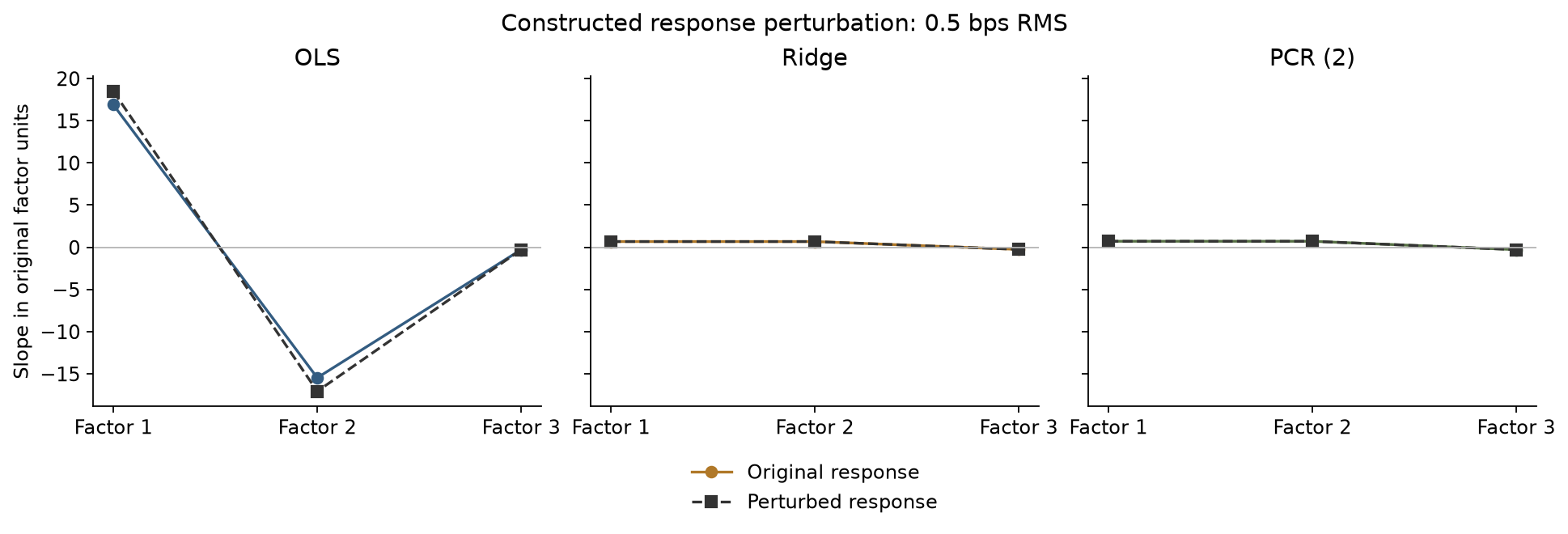
A constructed collinearity example isolates the mechanism. It is not historical ETF evidence. The observed six-factor design is much less extreme: its median rolling condition number is 2.94.
For centered target $y_c$, the estimates in standardized coordinates are
\[\widehat b_{OLS}=VD^+U^\top y_c,\] \[\widehat b_{ridge} =V\operatorname{diag}\!\left(\frac{d_j}{d_j^2+n\lambda}\right)U^\top y_c.\]The ridge objective is $\lVert y_c-Zb\rVert_2^2/n+\lambda\lVert b\rVert_2^2$. Dividing the loss by $n$ matters: the denominator contains $n\lambda$. The primary study fixes $\lambda=0.1$ and $n=60$. Principal-component regression provides another comparison, retaining four directions and discarding the remaining two. Ridge attenuates continuously; PCR makes a hard selection based on factor variance, which need not preserve explanatory value.
To report interpretable economic exposures, transform the slopes back:
\[\widehat\beta_j=\widehat b_j/s_j,\qquad \widehat\alpha=\bar y-\bar f^\top\widehat\beta.\]The intercept is unpenalized. A raw factor beta and a standardized slope answer different questions, so the exposure maps use the former. The SVD chapter shows the directional shrinkage and its relation to effective degrees of freedom.
Freeze the coefficients before evaluating another month
The first fit uses January 2007–December 2011, then evaluates January 2012. Move forward one month and repeat. Means, scales, and coefficients are always estimated on the previous 60 observations. The resulting 175 evaluations end in July 2026.
Here is a complete single-window example using the maintained modules. Run it in the research repository’s locked environment after acquiring the documented input cache:
1
2
3
4
5
6
7
8
9
10
11
12
13
14
15
16
17
18
19
20
21
22
23
24
import pandas as pd

from research.data import FACTORS, SECTORS, load_panel
from research.models import fit_factor_model

factors, excess_returns, audit = load_panel()
fund = next(ticker for ticker, name in SECTORS.items() if name == "Technology")
training_factors = factors.iloc[:60]
training_returns = excess_returns[fund].iloc[:60]

fit = fit_factor_model(
    training_factors,
    training_returns,
    method="ridge",
    ridge_lambda=0.1,
)
evaluation = factors.iloc[[60]]
reconstructed = fit.predict(evaluation)[0]
observed = excess_returns[fund].iloc[60]

print(pd.Series(fit.beta, index=FACTORS, name="Technology exposure"))
print(f"Evaluation month: {evaluation.index[0]}")
print(f"Observed excess return: {observed:.2%}")
print(f"Conditional reconstruction: {reconstructed:.2%}")
The reconstruction supplies the evaluation month’s realized factor returns, which were not known before the month. This tests whether earlier exposures explain a later observation; it is not a tradable return forecast. The retrospective factor vintage also does not recreate historical publication availability.
Challenge accuracy and stability separately
The primary loss averages squared errors equally across the nine sectors in each month. Compare ridge minus OLS on the same months and funds; negative differences favor ridge. A circular block bootstrap resamples 12-month blocks jointly across sectors and models, with 2,000 draws. It retains paired market shocks and some serial dependence. It does not account for every research choice or refit the models inside each draw.
Coefficient movement is a separate diagnostic. A smoother model can be consistently wrong, and a changing coefficient can reflect a genuine change in sector composition. Full-sample OLS intercepts therefore receive their own six-lag HAC uncertainty estimates and Holm adjustment across the nine tests. OLS p-values are not reused for biased ridge estimates.
The findings article brings these checks together. For hands-on work, explore the notebooks on return alignment, SVD geometry, and alpha uncertainty. For SVD applied to an asset-return covariance matrix, continue to SVD and portfolio risk.