
Technology and Utilities are both equity sectors, but their responses to common return patterns differ. Factor analysis makes those differences visible. The harder question is whether an exposure estimated from one sample remains useful in another.
In this study, ridge regression reduces subsequent-month reconstruction error by 2.24% relative to ordinary least squares. The paired uncertainty interval just excludes zero. That is evidence of a small historical gain for the chosen specification and universe. It is not a forecast of sector returns, an alpha discovery, or proof that smoother coefficients will always be better.
Research revision: 20 September 2026. The analysis now uses State Street Select Sector SPDR ETFs, with sector names on charts and tables. The executed report and result tables provide the calculations behind this article.
Read the economic exposure map
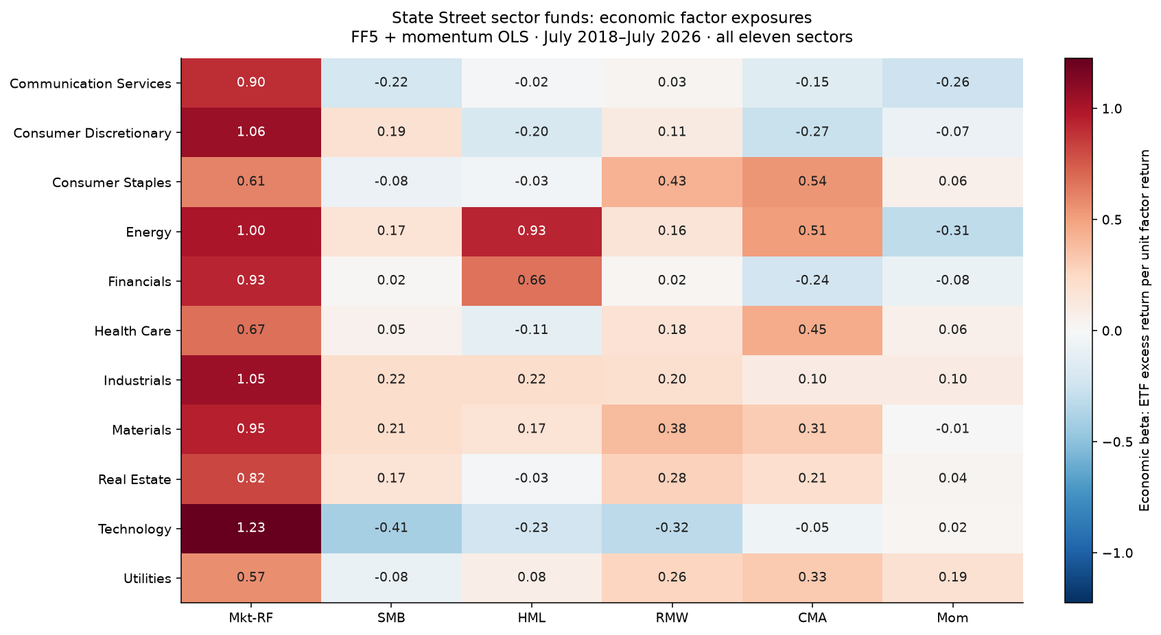
Descriptive full-sample OLS, July 2018–July 2026. Each row is a sector; each column is a factor-return sensitivity in economic units. This shorter eleven-sector sample is separate from the long-sample primary experiment below.
Each sector’s excess return is modeled using the market, size, value, profitability, investment, and momentum factors. The map estimates a market coefficient of about 1.23 for Technology, versus 0.57 for Utilities. Holding the other regressors fixed, a one-percentage-point market-factor move corresponds to fitted contributions of about 1.23 and 0.57 percentage points, respectively.
Energy and Financials have positive value-factor coefficients of approximately 0.93 and 0.66; Technology’s is approximately −0.23. These are conditional relationships over this sample, not portfolio weights or direct measurements of every company’s characteristics. The exposure table retains the full precision and source identifiers.
For a fixed model, the intercept, each contribution $\beta_j f_{j,t}$, and the residual add to the month’s realized excess return. Summing contributions through time does not create a compounded wealth attribution. Interpretation needs the return equation as well as the colors in the chart.
Give the long history and broader universe separate roles
The original nine State Street funds supply 235 monthly returns, January 2007–July 2026. After the first 60-month training window, the primary comparison has 175 evaluation months, January 2012–July 2026. All methods use the same dates and funds.
Real Estate and Communication Services have shorter fund histories. The eleven-sector extension starts in July 2018, giving 97 return months and only 37 rolling evaluations after training. Neither fund is assigned invented earlier returns. The data note documents launch dates, calendar alignment, and source checks.
For every evaluation month, coefficients use the preceding 60 months. The calculation then supplies the target month’s realized factors. This is conditional reconstruction: it tests estimated relationships after those factor returns become known. It does not supply an investment signal available before the month.
Does regularization improve the reconstruction?
The primary comparison fixes ridge’s penalty at 0.1 after training-window standardization. PCR retains four components. Neither setting is chosen by searching the evaluation results. Market-only and five-factor regressions provide simpler reference models.
| Model | Monthly reconstruction RMSE | RMS monthly beta movement |
|---|---|---|
| Market only | 3.477% | 0.0094 |
| Fama–French five factors | 3.037% | 0.0412 |
| Six-factor OLS | 3.037% | 0.0436 |
| Six-factor ridge, penalty 0.1 | 3.003% | 0.0348 |
| Four-component PCR | 3.322% | 0.0881 |
Primary nine-sector sample, January 2012–July 2026. Beta movement is computed within each model’s own coefficient set; the direct stability comparison is OLS against ridge using the same six factors. RMSE measures errors in monthly returns, not portfolio volatility.
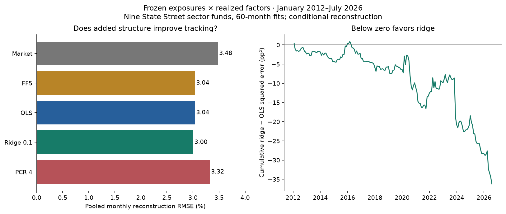
Ridge’s mean squared error is 9.0153 squared percentage points, compared with 9.2219 for OLS. The difference is −0.2067 pp², with a 95% paired 12-month block-bootstrap interval of [−0.4256, −0.0143]. The 2.24% headline is a relative reduction in squared error, not a 2.24-percentage-point return improvement. It corresponds to a much smaller change in RMSE, from roughly 3.037% to 3.003%.
The interval is conditional on the historical loss paths, with common sector shocks kept together in each resample. It does not capture uncertainty from universe selection, factor revisions, or unreported specification searches. Complete definitions are in the methods and findings.
Smoother coefficients are only part of robustness
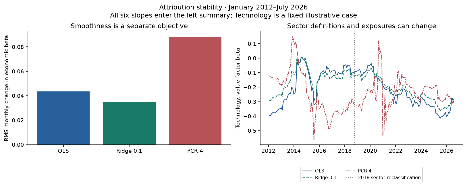
Ridge reduces coefficient movement, but aggressive compression is less successful. Four-component PCR has higher reconstruction error than six-factor OLS. Small-variance factor directions can still contain useful explanatory information.
The observed design is not catastrophically ill-conditioned: its median standardized condition number is 2.94, with a range of 2.42–3.74. The severe collinearity example in the implementation article explains a possible mechanism; it should not be mistaken for a description of every empirical window.
Stronger shrinkage also performs worse here. The study retains the declared penalty, window, and block-length sensitivities instead of replacing the primary result with whichever variant wins. Robustness means checking the limits of the conclusion, not finding another setting that makes the headline larger.
Neither an intercept nor a sector label is immutable
None of the nine full-sample OLS intercepts survives Holm adjustment at 5%. The intercepts use six-lag HAC uncertainty estimates, and their annual arithmetic display is 12 times the monthly coefficient. That is not a compounded strategy return. Even a significant intercept would be conditional on the factor model, the constant-beta approximation, and the data vintage; it would not by itself establish manager skill.
Sector composition can change for economic reasons. Real Estate separated from Financials in 2016, and Communication Services altered sector boundaries in 2018. The Financials distribution check confirms that two pinned Yahoo adjusted-price snapshots agree closely around the 2016 event and do not create a distribution-sized artificial crash. This is provider consistency, not an independent reconciliation to issuer NAV total returns.
The broader eleven-sector comparison gives a ridge-minus-OLS difference of −0.6428 pp², with interval [−1.0775, −0.1711], over July 2023–July 2026. That short path contains only about three 12-month blocks. The original nine on the same recent dates produce −0.7666 pp². Keeping both results visible separates a date-window change from adding two sectors; neither replaces the long-sample primary comparison.
Continue the research
The next evidence needed is an independent later sample, historical factor-release vintages, independently reconciled fund returns, and dated holdings that explain mandate changes. Those would test whether the observed gain travels beyond this retrospective study.
| Question to explore | Research note | Executed notebook |
|---|---|---|
| What does a factor map explain? | Economic exposures | Exposure analysis |
| Do earlier exposures explain later returns? | Rolling attribution | Chronological comparison |
| Is apparent alpha convincing? | Intercept uncertainty | Inference examples |
The original implementation and earlier iShares revision remain preserved. The State Street amendment followed observation of the earlier result; it is an explicit change of research scope, not an independent untouched experiment.