
A dealer receives a request for a bond quote. A more competitive price makes a fill more likely, but leaves less margin if the trade happens. A wider quote earns more per execution, until customers stop accepting it. The decision becomes harder when the relationship between price and demand changes while the dealer is still learning.
This project builds a small adaptive pricing engine around that problem. It combines an execution model whose fill probability decreases with dealer markup, a discounted online correction, and an optional randomized quoting rule. The data describe synthetic Treasury bond RFQs, so the findings concern this controlled setting.
The most useful result came from separating two ingredients often bundled together as “learning.” Under abrupt simulated demand shifts, discounted Thompson sampling reduces expected regret by 65.1% relative to frozen quotes. But a discounted greedy policy does better still. In this experiment, forgetting stale feedback explains more of the improvement than randomized exploration.
That conclusion also has a boundary: on the chronological holdout of the labeled history, the adaptive correction does not establish a predictive improvement. Understanding both results requires separating fill prediction, quote economics, and the value of a policy that chooses different prices.
Put both sides of the trade on the same scale
Let the side sign be $s=+1$ when the dealer sells at an ASK and $s=-1$ when the dealer buys at a BID. For quote $q$, current midprice $m$, and subsequent hedge mark $m^+$, define dealer markup $d$ and signed hedge movement $h$:
\[d=s(q-m),\qquad h=s(m^+-m),\qquad r=Y(d-h).\]Here $Y$ is one for a fill and zero for a miss. Positive $d$ means a dealer markup on either side: an ASK above mid or a BID below mid. Positive $h$ is an unfavorable hedge movement. Reward $r$ is measured in price points per 100 units of face value.
For example, an ASK of 100.07 against a mid of 100.00 has $d=0.07$. If the hedge mark subsequently rises to 100.02, the filled trade earns 0.05 price points under this markout convention. A BID of 99.93 against the same mid also has $d=0.07$; a fall in its hedge mark to 99.98 produces the same 0.05 reward.
The exact conditional expected-profit identity is
\[\mathbb{E}[r\mid x,d] =p(x,d)\{d-\mu_F(x,d)\}, \qquad \mu_F(x,d)=\mathbb{E}[h\mid Y=1,x,d],\]where $x$ is the information available before quoting and $p(x,d)$ is the fill probability. The hedge cost that matters is conditional on getting filled. A forecast of the unconditional hedge movement can miss that distinction.
The implemented rule approximates $\mu_F(x,d)$ with a context-only forecast $\mu(x)$. Forward validation selects a zero-change hedge forecast over the tested ridge regressions, so the primary objective becomes $d\,p(x,d)$. This selection supports a simple forecast within the experiment; it does not prove that execution and future price movements are independent.
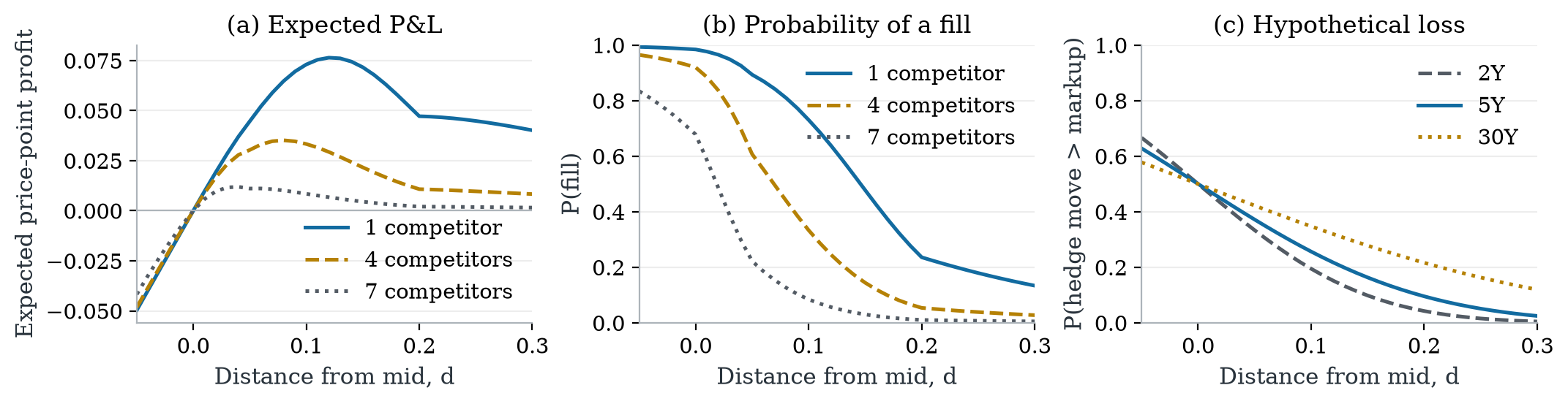
Fitted curves for a representative request. The first two panels vary competitor count while holding other inputs fixed. The third uses tenor-specific Gaussian hedge scales to show the probability that an adverse move exceeds the markup; it is not a measured loss probability conditional on a fill. All curves are model outputs from the synthetic sample.
Normalized units also avoid an unresolved notional convention in the supplied data. An alternative dollar interpretation rescales rewards without changing the optimum for an individual request. Summing normalized rewards gives equal weight to RFQ arrivals; it does not produce a notional-weighted portfolio return.
What the data can answer
The labeled sample contains 1,000 RFQs, five Treasury tenors from 2Y to 30Y, six counterparties, and an execution rate of 28.2%. There are another 100 requests without execution or hedge labels, plus ten requests for quote application. Predictions on those two sets are outputs, not independent performance estimates.
The audit removes 1,006 empty formatting rows and one non-data footer from the unlabeled sheet. Repeated timestamps in the labeled sample remain separate requests. They are ordered stably, and requests sharing a timestamp cannot use one another’s outcomes during historical replay.
Pre-trade features include tenor, side, notional, counterparty, competitor count, current midprice, and the candidate quote. Execution and the subsequent hedge mark are targets or outcomes, never demand inputs. Timestamp is used for ordering rather than as a demand feature.
The first 800 observations form the development sample; the final 200 form the chronological holdout. Model selection uses three forward folds with 340, 490, and 640 training observations, followed by a ten-row gap and 150 validation observations. Feature scaling and category encoding are fitted within each fold.
Actual fill and hedge timestamps are unavailable. The gap reduces adjacency, but cannot certify that every outcome would have been known before the next decision. The replay therefore makes an explicit feedback-timing assumption and permits only strictly earlier timestamps to update the current prediction.
Build an execution curve that respects price
The base model is logistic regression with linear context effects and constrained piecewise-linear price functions:
\[p_0(x,d)=\operatorname{sigmoid}\!\left( x^\top\beta+\sum_{j=1}^{7}b_jB_j(d) \right),\qquad b_j\leq 0,\] \[B_j(d)=\operatorname{clip}\!\left( \frac{d-k_j}{k_{j+1}-k_j},0,1 \right).\]The eight knots are $(-0.25,-0.05,0,0.05,0.10,0.20,0.35,0.55)$. Each ramp $B_j$ increases with markup, and its coefficient cannot be positive. Consequently, the model’s logit and fill probability cannot increase as the quote becomes more expensive for the customer, holding context fixed.
Context includes standardized log notional and competitor count, side, bond and counterparty indicators, a training-centered within-bond midprice, and a size–competition interaction. The additive price curve is deliberately compact; it does not allow unrestricted differences in price elasticity across contexts.
Forward validation selects the constrained spline with regularization parameter $C=1$: mean log-loss 0.4021, versus 0.4075 for the best constrained linear price model and 0.4116 for the four-leaf monotone boosted-tree benchmark. The tree model offers a nonlinear comparison; the online correction uses the monotone logistic family.
Quotes are selected by evaluating a finite grid of 71 markups, from −0.20 to 0.50 in steps of 0.01. No unique optimum or smooth profit surface is assumed. The application engine also restricts candidates to each bond’s observed 1st–99th percentile markup range. This reduces marginal extrapolation, but cannot establish that a particular quote is well supported for every counterparty and market state.
Adapt a small state while preserving the curve
Instead of repeatedly refitting the full model, the engine adds an eight-parameter contextual correction to its logit:
\[p_t(x,d;w)=\operatorname{sigmoid} \{\ell_0(x,d)+z(x)^\top w\}, \qquad w\approx\mathcal{N}(a_t,P_t).\]Here $\ell_0$ is the fitted base logit. The vector $z(x)$ contains an intercept, side sign, scaled log notional, scaled competitor count, and four bond indicators. It excludes quote distance. Every realization of the correction therefore preserves the monotonicity of the original curve and shares information across candidate prices. The tradeoff is that this state can change contextual demand levels, but cannot directly learn a new price slope.
At each RFQ arrival, the filter discounts its accumulated evidence toward a zero-mean prior. With precision $A=P^{-1}$ and prior precision $\lambda I$,
\[\begin{aligned} A^-&=\gamma A+(1-\gamma)\lambda I,\\ P^-&=(A^-)^{-1},\\ a^-&=P^-\gamma A a. \end{aligned}\]The implementation uses $\lambda=4$ and selects $\gamma=0.97$ from three candidate forgetting factors using development data. The implied evidence half-life is $\log(1/2)/\log(0.97)=22.8$ arrivals. That is a weighting convention, not a measured time to recover from a demand shock.
The policy then draws one contextual adjustment from the working Gaussian:
\[u\sim\mathcal{N}\!\left(z^\top a_t,\tau^2z^\top P_tz\right),\] \[d_t=\underset{d\in\mathcal{D}(x)}{\operatorname{arg\,max}}\; \operatorname{sigmoid}\{\ell_0(x,d)+u\}\{d-\mu(x)\}.\]The same draw applies to every candidate price for that request. There are no independent posteriors for the 71 grid points. Temperature $\tau=0.35$ gives the tempered Thompson-sampling policy; setting $\tau=0$ gives discounted greedy.
When a binary outcome arrives, a local-curvature Gaussian update adjusts the mean and covariance using the stored context and chosen quote. This is an approximate filter conditional on a fixed base model. Its covariance does not include uncertainty in the original fitted demand curve, and it supplies neither an exact Bayesian posterior nor an inherited regret guarantee.
Feedback is applied once per RFQ identifier. Pending requests, filter state, and random-number state can be saved together for restart. Delayed outcomes receive full likelihood weight on receipt: discounting follows arrival count and receipt time, rather than elapsed clock time or the age of the original request.
Historical prediction does not show an adaptation gain
The chronological holdout evaluates probabilities at the prices actually quoted. Lower log-loss and Brier score are better; higher AUC indicates better ranking of fills above misses.
| Model | Log-loss | Brier score | AUC |
|---|---|---|---|
| Frozen monotone spline | 0.3504 | 0.1148 | 0.9039 |
| Monotone boosted trees | 0.3665 | 0.1208 | 0.8944 |
| Constant development fill rate | 0.5838 | 0.1973 | 0.5000 |
| Discounted logged correction | 0.3530 | 0.1145 | 0.8989 |
| Stationary logged correction | 0.3684 | 0.1203 | 0.8891 |
The discounted correction’s log-loss is slightly worse than the frozen model’s. Its paired difference is +0.00266, with a 95% circular block-bootstrap interval of [−0.01760, +0.02198] using blocks of ten observations and 1,500 resamples. Block lengths five and twenty also produce intervals containing zero. The small Brier improvement does not overturn this inconclusive comparison.
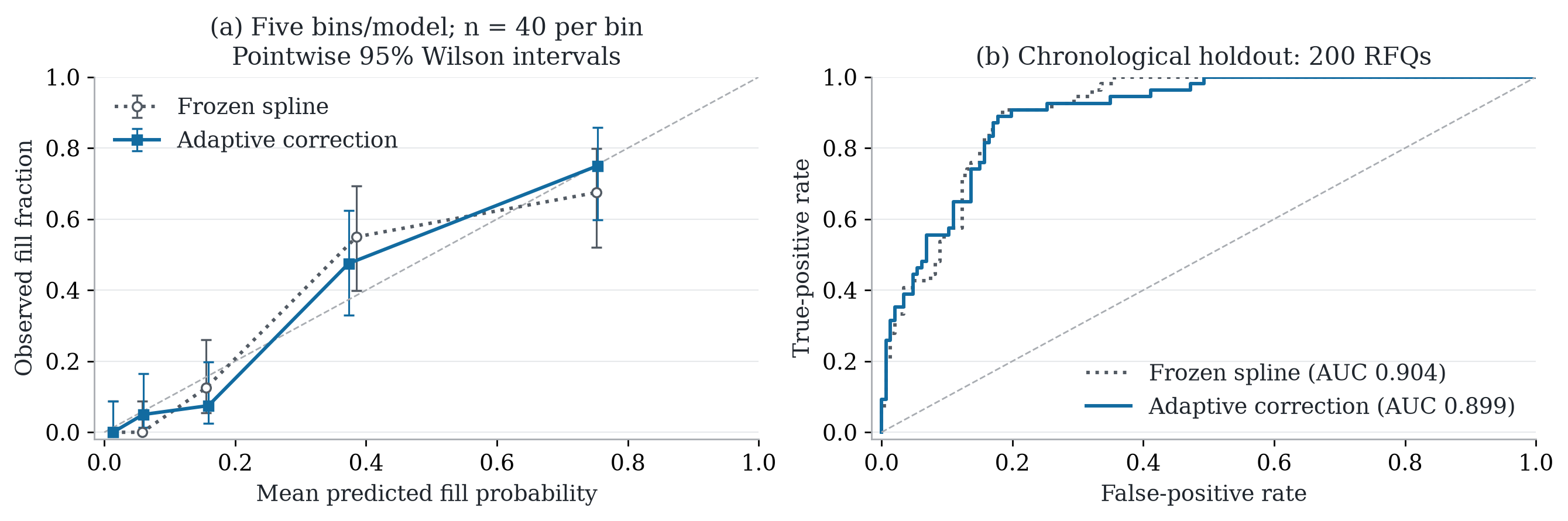
Five equal-count calibration bins are formed separately for each predictor. Wilson intervals describe uncertainty in the observed fill fractions but do not adjust for serial dependence. The ROC panel measures discrimination at logged actions; neither panel evaluates the profit of newly selected prices.
The zero-change hedge forecast has holdout RMSE 0.1871 price points and MAE 0.1451. Its nominal 90% Gaussian intervals cover 91.5% of the observed changes. Those unconditional diagnostics cannot establish accuracy after conditioning on a fill. The additional 100 unlabeled requests receive final-model probabilities, but have no observed outcomes against which to score them.
A new quote needs a new outcome model
Suppose the history records a fill at markup 0.03. A candidate policy would have quoted 0.10. Reusing the historical fill as if the customer accepted 0.10 would invent a counterfactual outcome. Good prediction at logged prices does not solve this problem.
The project therefore studies policy learning in a separate simulator. For each of 30 paired seeds, it resamples 1,800 contexts from development data. Policies share the same contexts, uniform execution draws, and hedge shocks within a seed. Each learner observes only its chosen action’s binary outcome. Only the evaluator can see the complete expected-reward surface.
Four environments expose different behaviors:
| Environment | Demand and feedback assumptions |
|---|---|
| Stationary | The fitted base curve is the true demand curve, making frozen pricing an oracle by construction. |
| Abrupt shifts | The base logit receives offsets 0, −1.5, and +1.5 across three blocks of 600 arrivals. Policies do not know the changes. |
| Misspecified | A probit link, time-varying price slope, and additional contextual interaction depart from the fitted correction family. |
| Delayed feedback | The abrupt-shift environment returns outcomes after 25 arrivals, versus one arrival in the other scenarios. |
All environments use independent, zero-mean Gaussian hedge shocks with standard deviation 0.18. They isolate demand adaptation and do not test learning a changing conditional hedge cost. Simulation uses the entire global quote grid, whereas the application engine adds the bond-specific support restriction.
The comparison metric is cumulative expected regret: the sum of expected profit forgone relative to the best grid quote in each simulated context. With the simulator’s zero expected hedge movement,
\[R_T=\sum_{t=1}^{T} \left\{\max_{d\in\mathcal D}p_t(d)d-p_t(d_t)d_t\right\}.\]It is measured in summed price points per 100 face. It is not a realized return, a Sharpe ratio, or a percentage gain in trading profit.
Forgetting explains the main simulated improvement
The mean expected regrets over 1,800 requests are:
| Policy | Stationary | Abrupt shifts | Misspecified | Delayed feedback |
|---|---|---|---|---|
| Frozen | 0.000 | 7.405 | 68.123 | 7.405 |
| Stationary Thompson sampling | 0.267 | 8.886 | 69.293 | 9.054 |
| Discounted greedy | 0.467 | 2.338 | 43.277 | 2.809 |
| Discounted Thompson sampling | 0.697 | 2.588 | 43.172 | 3.017 |
| Epsilon greedy | 1.744 | 3.562 | 43.507 | 4.021 |
Lower is better. Epsilon greedy uses the discounted greedy rule except for 5% exploration among nonnegative-margin actions. The stationary environment’s zero frozen regret follows from its construction.
Under abrupt shifts, discounted sampling reduces regret from 7.405 to 2.588, or 65.1%. Its paired difference from frozen pricing is −4.817, with a 95% Student-$t$ interval over seeds of [−4.960, −4.674].
But discounted greedy reaches 2.338. Turning sampling on adds 0.250 regret, with interval [0.206, 0.294]. The benefit of discounting survives when randomized exploration is removed. That ablation is the reason to credit forgetting as the principal mechanism in this environment.
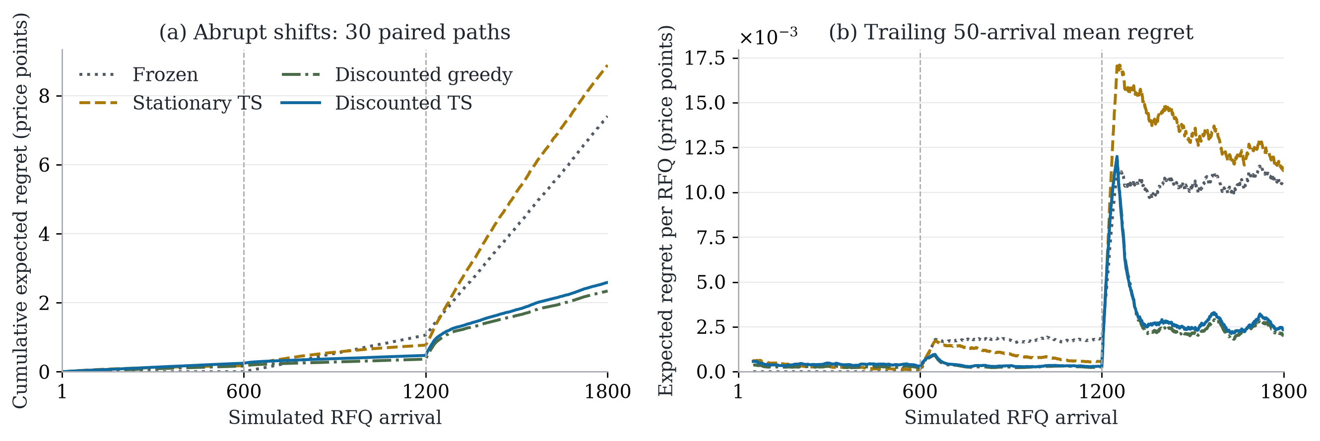
Means over 30 paired simulation seeds. Vertical lines mark regime boundaries after arrivals 600 and 1,200. The trailing 50-arrival mean is a descriptive display, not an input to the policy. These paths do not estimate recovery speed in a market.
The other environments qualify the result. With delayed feedback, discounted sampling’s regret rises to 3.017, again above discounted greedy. Under misspecification, sampling slightly improves the point estimate relative to greedy, but their paired difference of −0.105 has interval [−0.596, +0.387]. The much larger absolute regret in that environment exposes the limitations of an online state that cannot directly relearn the price slope.
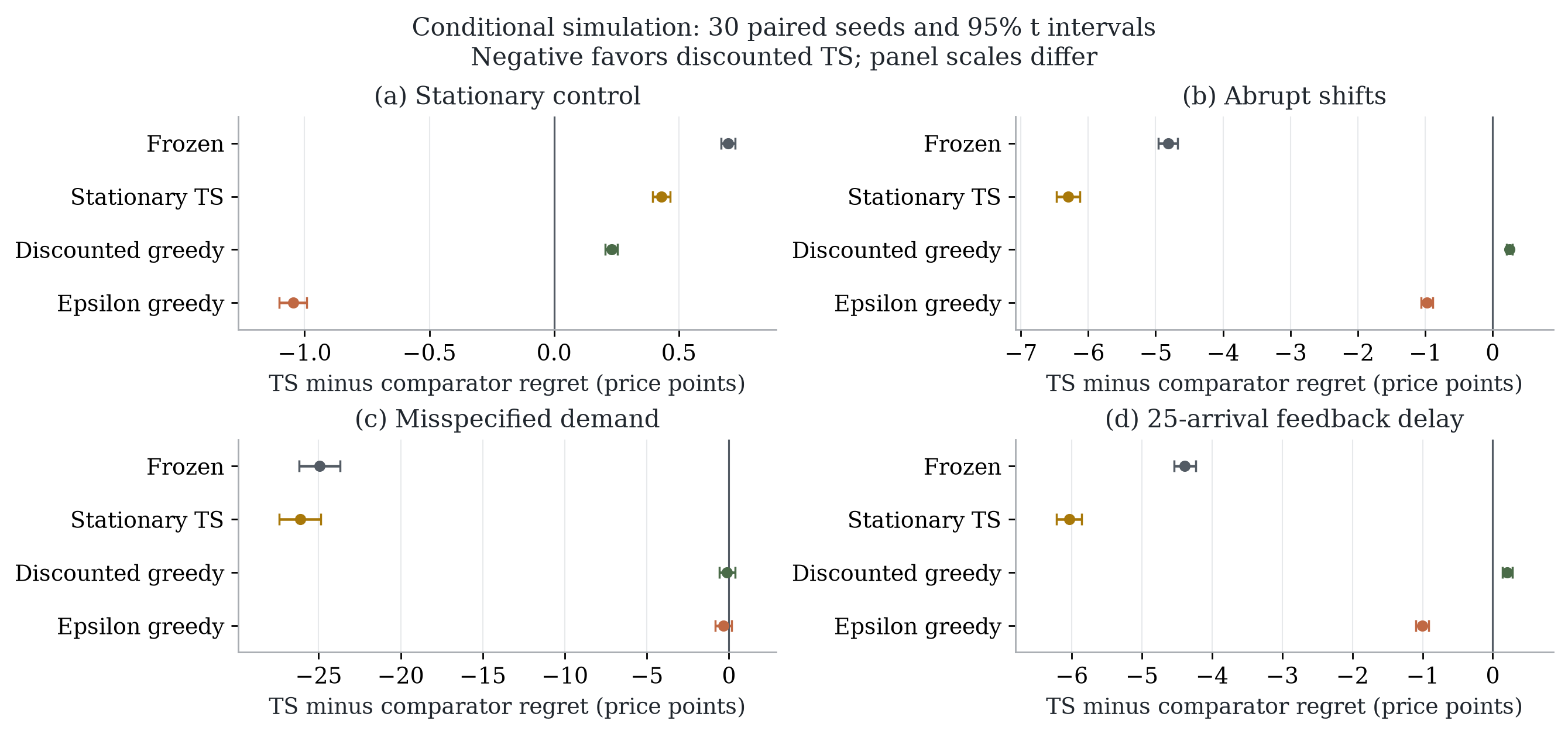
Negative differences favor discounted Thompson sampling. Bars show 95% Student-$t$ intervals over 30 paired seeds; panel scales differ. These intervals describe Monte Carlo uncertainty conditional on the fitted simulator. They do not include uncertainty about real demand or the original training sample, and the comparisons are not adjusted for multiplicity.
The matched stationary control also matters. When the frozen model already knows the true expected-reward surface, estimation noise and exploration impose costs. This is a useful implementation control, but it is not independent evidence that a frozen policy would be optimal in a real market.
A good execution model still needs the right objective
The final model is refit on all 1,000 labels after evaluation and produces deterministic expected-profit quotes for ten unlabeled requests. Their selected markups range from 0.03 to 0.12. The absolute quote follows $q=m+sd$; markup uses the 0.01 grid, while absolute prices can retain three decimals from the supplied midprice. No fills or hedge outcomes are known for these decisions.
The important sensitivity is what happens when fills carry an adverse hedge cost. Holding the execution curve fixed, imposing conditional costs of 0.02, 0.05, or 0.10 price points moves the profit-optimal quotes outward in these examples. These are imposed scenarios rather than estimated causal effects. Development residuals already suggest why the distinction deserves attention: mean signed hedge residuals are 0.0336 on filled requests and 0.0138 on misses. Context mix could explain that association, so the difference does not identify adverse selection.
The project also includes an illustrative contest score with different incentives: a negative hypothetical margin earns −1 even without execution, a safe fill earns +1, and a safe miss earns −0.25. Ignoring ties, let $L=\Pr(h>d)$ and $J=\Pr(Y=1,h\leq d)$. Then
\[\mathbb E[S]=1.25J-0.25-0.75L, \qquad \max(0,p-L)\leq J\leq\min(p,1-L).\]The point proxy assumes independence, $J=p(1-L)$, while the bounds leave the dependence unspecified. Optimizing this score can favor a wide quote that nearly guarantees a safe miss. That behavior follows the score’s incentives and should not be interpreted as expected-profit maximization.
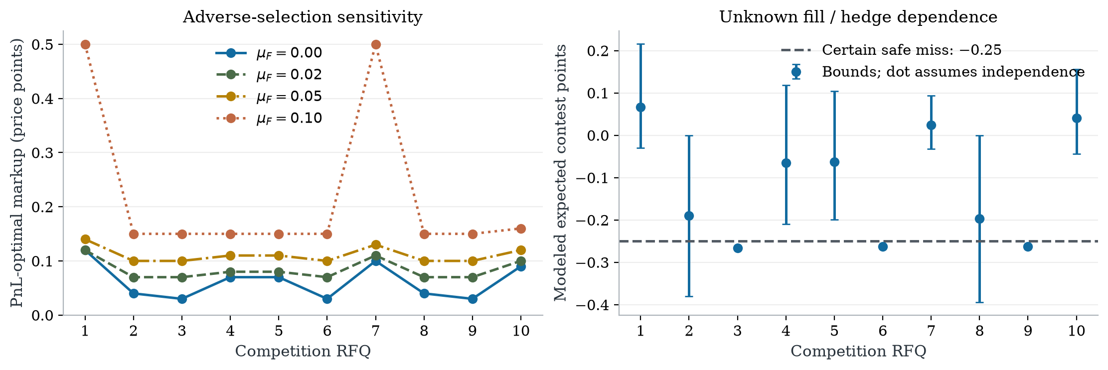
Left: expected-profit decisions for ten unlabeled application requests after imposing a conditional hedge cost. Right: expected-score bounds evaluated at the independence-proxy decisions. The figure labels these requests “Competition RFQ.” The bounds concern unknown dependence given the marginal models, not sampling uncertainty. Neither panel shows realized trading results.
What this changes about the next experiment
The engine provides a compact way to update demand while keeping price responses economically coherent. Its most persuasive simulated improvement comes from discounting old observations. The historical sample provides no clear reason to prefer the adaptive predictor, and the simulation provides no consistent reason to prefer sampling over discounted greedy.
A prospective test would need to log contexts, candidate prices, selected-action probabilities, model states, fill times, and hedge-mark times. Those records would allow feedback timing and action overlap to be checked before attempting policy evaluation. Inventory, fees, persistent price impact, and customer or competitor responses would also need to enter the economic model when they affect decisions.
The next useful comparison is therefore specific: can a demand correction improve quote value after actual outcome delays and conditional markouts are accounted for? Keeping exploration optional makes that question easier to test. The present results support an interpretable implementation and a controlled study of adaptation; they do not establish live-market profitability.
Inspect the numerical evidence
These compact tables accompany the article:
- Chronological holdout metrics.
- Block-bootstrap sensitivity for adaptive minus frozen log-loss.
- Simulation summaries across policies and environments.
- Paired simulation regret differences and intervals.
The article adapts the project’s completed research manuscript and executed notebook. Figures are unchanged copies of the original computed outputs, and the tables retain their reported precision. Historical prediction and synthetic policy experiments remain separate throughout; the additional application requests have no observed outcomes.