
Suppose a bond portfolio becomes less volatile after adding signals from its issuers’ equity prices and financial statements. That sounds like a useful extension: another market may reveal information that credit investors have missed.
But a quieter portfolio does not, by itself, justify a more complicated process. Reducing the original positions would also reduce risk. The harder question is whether the new information earns its place after that simpler alternative is available.
That comparison changed how I interpret this corporate-bond factor study. A fixed combination of bond and issuer-equity signals does not establish a reliable advantage over a bond-only portfolio scaled using prior volatility. Yet the aggregate result hides an interesting split: equity momentum has positive conditional alpha, while equity value has negative conditional alpha. Understanding both findings is more useful than treating either one as the verdict on equity information in credit.
An equity signal can still be a bond trade
Equity and debt are claims on the same business, but they do not share the same payoff. Shareholders participate in upside after creditors are paid; bondholders care about promised payments, recovery, and the changing probability of distress. A characteristic that helps explain stocks therefore need not transfer to bonds in the same direction.
Issuer equity momentum offers one plausible hypothesis. A rising share price may reflect improving information about the issuer before that information is fully reflected in its bonds. But common risk or stale bond prices could produce a similar historical pattern. A positive factor estimate cannot identify which explanation is right.
I examine six existing long–short corporate-bond portfolios, grouped by the information used to sort their holdings:
| Bond characteristics | Issuer equity characteristics |
|---|---|
| Higher credit spread | Stronger equity momentum |
| Stronger bond momentum | Higher book-to-market equity |
| Lower bond-return volatility | Higher gross profitability relative to assets |
The equity-derived group also holds bonds. It does not buy stocks, and combining the groups does not create a conventional stock–bond allocation. Each group is an equally weighted average of three published factor-return series; the combined portfolio assigns half to each group, or one-sixth to each signal.
All reported returns are gross long–short factor P&L per unit of fixed long-side reference notional, not returns on a funded portfolio.
The common sample contains 231 months, September 2002–November 2021. Its primary returns come from the DFPS file distributed through Open Source Bond Asset Pricing. DFPS denotes the Dick-Nielsen, Feldhütter, Pedersen, and Stolborg return source. These are TRACE-derived returns paired with externally constructed characteristics, not a new transaction-level reconstruction performed here. The data chapter explains that boundary. This is historical research ending in 2021, not a current-market backtest.
A reproducible number can describe the wrong trade
Before interpreting the combination, I reproduced the archive’s database-comparison table: 341 factors and 12 statistics per factor. All 4,092 values match to numerical precision. That establishes that I can reproduce the supplied summary calculations. It does not independently validate the underlying transaction cleaning.
The next question is what each column actually means. The provider marks some factors whose returns were reversed to orient their historical premium positively. Replication must retain those signs. Testing a stated economic idea requires a separate mapping from the stored return to the intended long and short positions.
For this study, that means undoing the marked reversals for bond momentum and equity profitability, and reversing the unstarred high-volatility factor to test a low-volatility hypothesis. The result is economically consequential: the combined portfolio’s Sharpe is 0.66 using the source-oriented returns, versus 0.05 under the study’s economic directions. Its annual arithmetic mean changes from 3.71% to 0.13%.
Those are different exposures. The gap is not a pure estimate of look-ahead bias, nor evidence that every source factor is invalid. It shows why a familiar factor label cannot substitute for checking the actual trade. The signal mapping and replication details keep both calculations visible.
Diversification is visible; its incremental value is less clear
Under the economic directions, combining the two groups reduces full-sample annualized volatility from 3.47% for bond-only to 2.53% for the combination. The annual mean increases from −0.12% to +0.13%, but the paired mean difference has a 95% interval from −0.41 to +0.90 percentage points. The observed increase is uncertain.
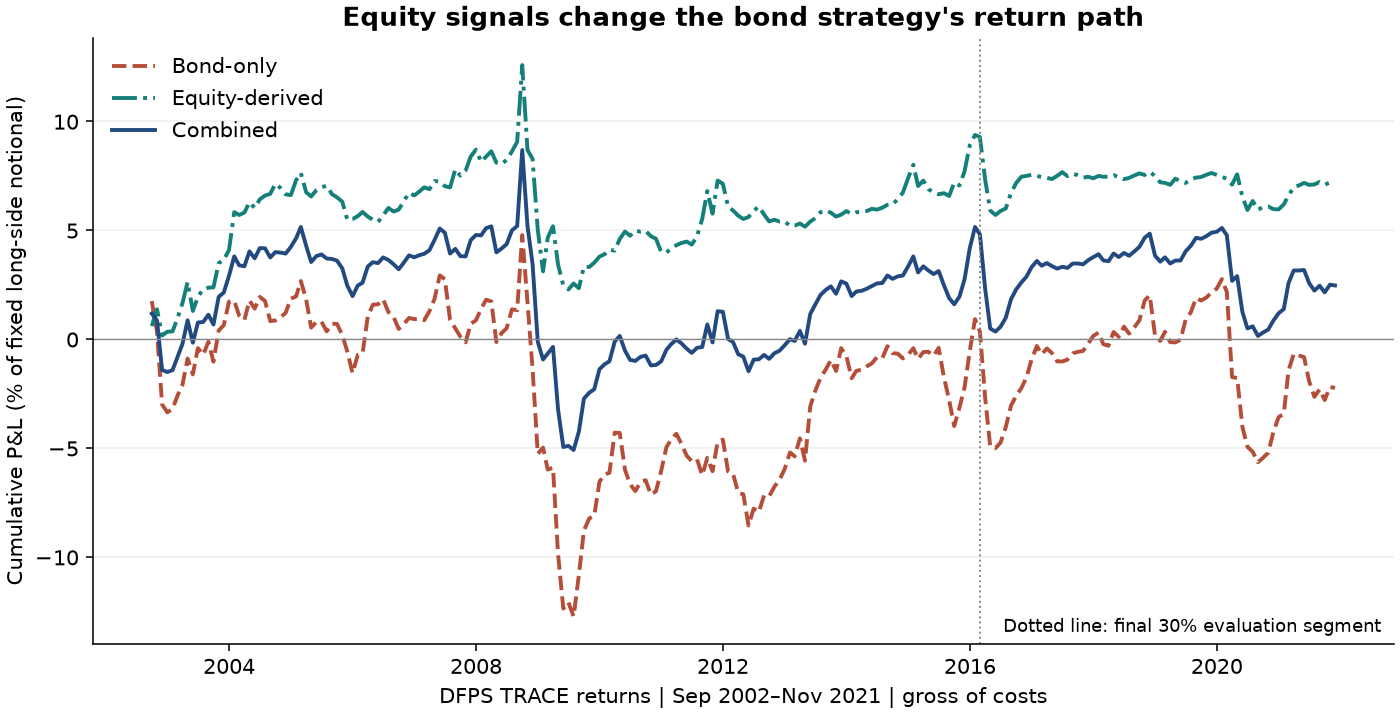
Original portfolio paths, September 2002–November 2021. The chart sums monthly gross factor returns as a percentage of fixed long-side notional; it is not compounded wealth or funded NAV. It does not include the scaled control introduced below. The later segment is a chronological diagnostic on already known, revised history.
The correlation structure helps explain the quieter portfolio. Credit spread and low volatility have a monthly correlation of −0.88; equity momentum and equity value correlate at −0.76. Six equally weighted names are not six independent sources of information. Some exposures substantially offset one another.
This raises the allocation question more sharply: how much of the apparent improvement requires the equity signals, and how much can be obtained by taking less bond-factor risk?
Compare the addition with a smaller original position
Let $B_t$ be the bond-only return and $C_t$ the combined return. Construct a control that scales the bond portfolio using volatility estimated over the preceding 60 months:
\[w_t=\min\!\left(1,\max\!\left(0, \frac{\widehat\sigma(C_{t-60:t-1})}{\widehat\sigma(B_{t-60:t-1})} \right)\right),\qquad B_t^{control}=w_tB_t.\]The current month’s return cannot affect its weight. The cap prevents scaling the bond sleeve above its original notional. Unused reference notional contributes zero excess P&L. Cash yield, collateral returns, and financing are not modeled. This is a diagnostic control with comparable intended risk; prior volatility estimates do not guarantee identical realized risk.
Every comparison involving this control excludes the first 60 months as a warmup. In the original later segment, February 2016–November 2021, the results are:
| Portfolio | Annual arithmetic mean | Annualized volatility | Sharpe |
|---|---|---|---|
| Bond-only | −0.54% | 3.13% | −0.173 |
| Bond-only, scaled using prior volatility | −0.32% | 2.17% | −0.149 |
| Combined bond and equity-derived signals | −0.46% | 2.07% | −0.223 |
The combination is slightly less volatile, but it loses more than the scaled control over these 70 months. Its paired Sharpe difference is −0.074, with a 95% six-month-block interval of [−0.242, +0.109]. The interval includes zero. This is not convincing evidence of an improvement or statistically established underperformance.
Across the longer post-warmup period, September 2007–November 2021, the Sharpe difference is slightly positive, with an interval that also includes zero. The complete comparison retains both periods. The paired block-bootstrap intervals condition on the realized control weights and return paths; they do not correct for research selection.
How much extra cost could the addition support?
An additional signal family needs an economic benefit large enough to justify its implementation. One transparent starting point is the mean difference between the combination and its control. Interpret it as the additional constant annual cost the combination could bear before surrendering its estimated return advantage.
A basis point (bp) is 0.01 percentage point. The HAC uncertainty intervals allow for changing return variance and serial correlation through six monthly lags.
| Combined minus scaled bond control | Incremental mean | 95% HAC interval (bps/year) |
|---|---|---|
| September 2007–November 2021 | +9.17 bps/year | [−33.65, +51.98] |
| February 2016–November 2021 | −13.71 bps/year | [−51.62, +24.19] |
Negative headroom should stay negative. In the later segment, the combination is already behind before assigning it extra costs. The study does not observe turnover, bid–ask spreads, or borrowing costs, so these numbers are not transaction-cost estimates. They also differ from the combination’s total gross break-even hurdle.
The exploratory amendment uses 50 bps per year as an illustrative materiality threshold, not a measured cost requirement. The later interval’s upper bound is below that threshold. Under these assumptions, the data do not support a 50-bps improvement. Because the interval still includes zero, they do not establish equivalence or prove that the combination must perform worse in the future.
The average conceals opposing issuer signals
The allocation result does not settle whether any individual equity signal contains useful information. To examine that question, I regress each equity-derived bond factor on the three bond factors, the corporate-bond market excess return, and a Treasury term factor:
\[E_{j,t}=\alpha_j+\gamma_j^\top f_{bond,t} +\beta_{M,j}MKTB_t+\beta_{T,j}TERM_t+\epsilon_{j,t}.\]Here the intercept asks what remains unexplained by this particular linear return model. The full-sample annualized estimates are:
| Equity-derived target | Conditional alpha | 95% HAC interval |
|---|---|---|
| Momentum | +3.93% | [+2.04%, +5.81%] |
| Value | −2.33% | [−3.97%, −0.69%] |
| Profitability | +0.20% | [−1.33%, +1.73%] |
| Equal-weight equity composite | +0.60% | [−0.10%, +1.29%] |
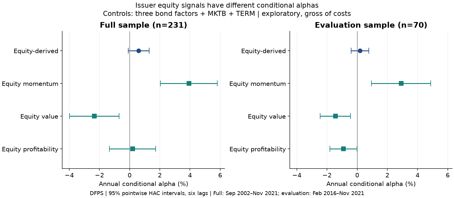
DFPS returns; full sample September 2002–November 2021 and later segment February 2016–November 2021. Intercepts are annualized arithmetically and gross of costs. Bars show pointwise 95% six-lag HAC intervals under the five stated controls. Open the figure to inspect both panels at full resolution.
Momentum and value pull in opposite directions. Their average, together with profitability, leaves the composite with an inconclusive intercept: p = 0.092. Momentum’s later alpha remains positive at 2.91%, and it passes the 5% Benjamini–Hochberg multiple-testing adjustment across the four targets in both segments.
The conditioning set matters. Momentum’s full-sample standalone mean is only 0.63%; its larger conditional alpha describes a fitted subtraction of correlated exposures. The hedge coefficients are estimated contemporaneously within each sample. That 3.93% is therefore not a realized return from an implementable hedged strategy. The original market-and-TERM-only regression also gives different inference; neither model’s testing adjustment corrects every prior research choice.
These diagnostics were added after examining the original results. Selecting momentum alone, or reversing value because its estimated alpha is negative, would create a new strategy requiring new validation. It would not rescue the original combination.
The next experiment needs prices one could actually trade
The useful lead is more specific than “equity factors work in credit”: does issuer equity momentum predict bond repricing within comparable credit-risk groups, or does the effect reflect risk and stale price observations?
Answering it requires a bond-level panel with dated issuer links, characteristic availability, cash flows, and executable entry prices. Bond-only and bond-plus-equity models should face the same eligible securities, exposure constraints, and cost accounting. Fresh-price subsets and entry delays would help distinguish information transmission from a return that disappears before execution. Shifting an aggregate factor-return series by one month cannot reproduce that test.
For this experiment, comparisons should be across issuers within comparable risk groups. An issuer equity signal is shared by that issuer’s bonds in a given month; issuer-by-month fixed effects would absorb it. That is a different question from relative value between two bonds of the same issuer.
The follow-on design is specified but unrun. The completed study supports a disciplined allocation decision: the fixed combination has not earned its additional complexity, while the component analysis identifies a narrower hypothesis worth testing with new evidence.
Evidence and further reading
The executed research notebook connects the calculations, figures, and sensitivity checks. Detailed notes cover factor direction, portfolio construction, and uncertainty and cost headroom. Alternative OSBAP and ICE return files give similar broad conclusions, but share signals and historical information; they are dependent source checks, not independent replications.
The research builds on Dick-Nielsen and coauthors’ corporate-bond factor framework and Dickerson, Nozawa, and Robotti’s work on trading delays. The source register credits the data and portfolio constructors and distinguishes their findings from the calculations here. Figures are original project outputs from those author-released inputs; source-specific terms remain described in the data notice. The article uses the project’s 16 September 2026 research revision, with its historical sample and exploratory status intact.