
A portfolio with ten ETFs does not necessarily contain ten independent bets. Several sector funds may rise and fall with the same equity-market shock. A collection of bond ETFs may share much of its interest-rate exposure. The portfolio looks diversified by ticker, while its returns tell a more concentrated story.
Singular value decomposition (SVD) gives us a way to examine that story. Principal component analysis (PCA) turns the decomposition into a statistical description of the directions in which returns vary most. Those directions can help us understand exposures, estimate risk, and construct systematic portfolio rules.
In this post, I work from the matrix representation to a practical ETF experiment. The aim is to explain what SVD computes, how it connects to PCA, and what additional decisions are needed to use either in systematic investing. The final experiment asks whether a PCA risk model improves portfolio construction relative to simpler alternatives.
Research revision: 20 September 2026. This expands my original 2024 SVD post. The matrix diagrams and sector example remain the starting point; the revised implementation adds explicit training windows, realistic timing, trading costs, and uncertainty. The code and executed notebooks are in the project repository.
1. Represent the investment universe as a matrix
Suppose we collect $T$ daily returns for $N$ ETFs. Arrange them in a matrix $R\in\mathbb{R}^{T\times N}$:
\[R= \begin{bmatrix} r_{1,1} & r_{1,2} & \cdots & r_{1,N} \\ r_{2,1} & r_{2,2} & \cdots & r_{2,N} \\ \vdots & \vdots & \ddots & \vdots \\ r_{T,1} & r_{T,2} & \cdots & r_{T,N} \end{bmatrix}.\]Each row is a trading date; each column is an asset. Three years of observations might give roughly 750 rows. With ten ETFs, the matrix is approximately $750\times10$.
For PCA, first subtract each asset’s mean return:
\[X=R-\mathbf{1}\bar r^\top.\]Now the columns of $X$ have zero sample mean. Centering matters because PCA describes variation around the mean. An SVD of raw, uncentered returns is still mathematically valid, but it describes an uncentered second moment rather than the sample covariance used below.
In a backtest, the sample means must come from the training window. The same rule applies to volatility estimates, factor loadings, and every other quantity we fit.
2. SVD: decompose the matrix into directions and magnitudes
For a real matrix, SVD writes
\[X=USV^\top.\]I use $S$ for the singular-value matrix and reserve $\Sigma$ for covariance. The three pieces have different jobs:
- The columns of $V$ are orthonormal directions in asset space.
- The diagonal entries of $S$ are nonnegative singular values, ordered from largest to smallest.
- The columns of $U$ are orthonormal directions in observation space, which here means time.
A general linear transformation does not preserve every orthogonal pair of directions. SVD identifies special orthogonal input directions whose nonzero images are also orthogonal, with each direction stretched by its own singular value.
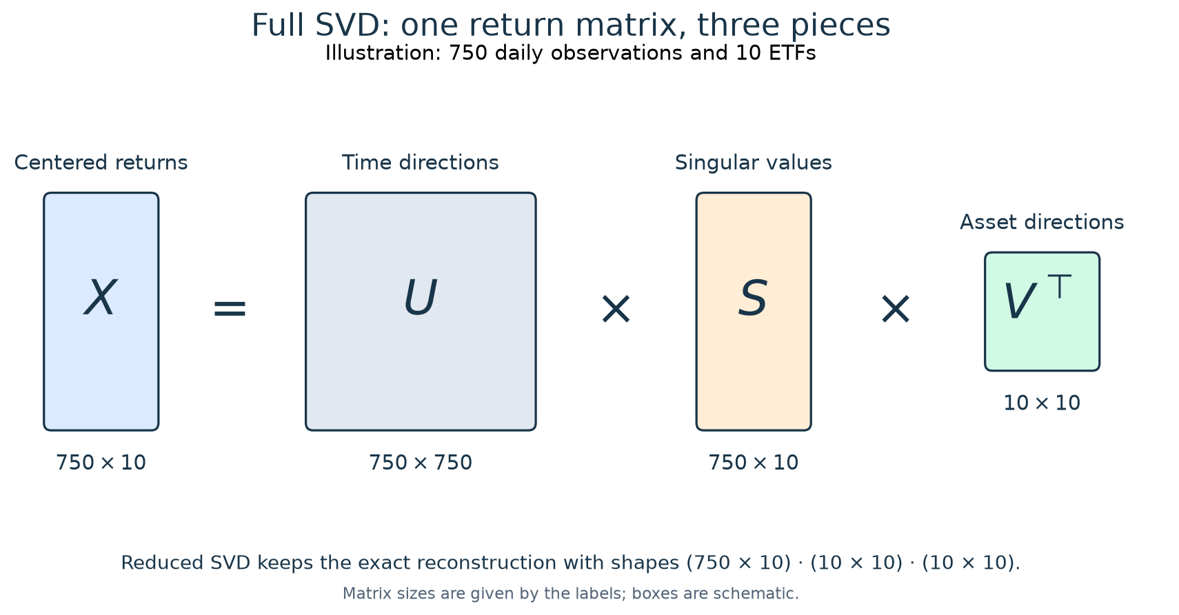
Figure 1. Full SVD, using the original post’s illustrative dimensions. The shapes are schematic; the dimension labels define the multiplication. The full decomposition reconstructs $X$ exactly.
For the $i$th pair of directions,
\[Xv_i=s_i u_i.\]This equation is the most useful way to read the decomposition. Start with a direction across assets, $v_i$. Apply the return matrix to it. The result is a pattern through time, $u_i$, with magnitude $s_i$. Equivalently, each component contributes an outer product:
\[X=\sum_i s_i u_i v_i^\top.\]A large singular value identifies a direction with a large contribution to the matrix’s total squared magnitude. For centered returns, that is directly connected to variance.
Full and reduced SVD
The large $U$ matrix in Figure 1 is useful for understanding the full decomposition. It is usually unnecessary for this application. With $T\geq N$, the reduced form is:
| Matrix | Full SVD | Reduced SVD |
|---|---|---|
| $U$ | $T\times T$ | $T\times N$ |
| $S$ | $T\times N$ | $N\times N$ |
| $V^\top$ | $N\times N$ | $N\times N$ |
Both forms reconstruct the same $X$. Reduced SVD removes unused dimensions without discarding any component needed for reconstruction. NumPy returns the singular values as a one-dimensional array rather than constructing $S$; full_matrices=False selects the reduced form. The NumPy documentation provides the exact shape and reconstruction conventions.
Reduced SVD and truncated SVD are different: reduction changes the representation’s size; truncation deliberately keeps fewer components and can lose information.
3. PCA: find the directions with the most variance
PCA gives a statistical interpretation to the decomposition of centered data. For a unit-length asset direction $v$, the score series is $Xv$, and its sample variance is
\[\operatorname{Var}(Xv)=v^\top\widehat\Sigma v, \qquad \widehat\Sigma=\frac{X^\top X}{T-1}.\]The first principal direction maximizes this variance subject to $v^\top v=1$. The next one maximizes variance subject to being orthogonal to the first, and so on.
Substituting the reduced SVD gives
\[\widehat\Sigma =V\frac{S^2}{T-1}V^\top.\]The connection follows immediately:
\[\lambda_i=\frac{s_i^2}{T-1}, \qquad Z=XV=US.\]The columns of $V$ are the principal directions, often called loadings. The columns of $Z$ are the component score series through time. $U$ alone contains normalized time patterns; $US$ restores their scale.
The score series are uncorrelated within the fitted sample because their sample covariance is diagonal. Uncorrelated does not mean statistically independent, and it does not guarantee that these relationships persist out of sample. A component may resemble broad equity-market exposure, but its economic interpretation requires inspecting the loadings and the underlying assets.
A loading vector can also flip sign without changing the decomposition: changing the signs of both $u_i$ and $v_i$ leaves their product unchanged. A sign change in a rolling chart is therefore not automatically a change in market structure.
Centering and scaling answer different questions
Covariance-space PCA centers returns and keeps their original units. More volatile assets can have more influence on its leading directions. Correlation-space PCA additionally divides each asset by its training standard deviation, giving equal unit variance to the inputs.
Neither choice is universally preferable. If standardizing, a covariance model must be mapped back to return units before calculating portfolio risk. This project uses covariance-space PCA as its primary specification and tests correlation-space PCA as a sensitivity check. Standard PCA centers but does not automatically standardize the inputs.
4. Keep the strongest common patterns
Using only the first $k$ components gives
\[X_k=U_kS_kV_k^\top.\]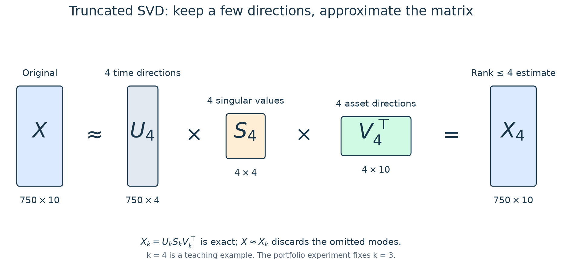
Figure 2. Keeping four components gives matrices of size $(750\times4)$, $(4\times4)$, and $(4\times10)$. Their product is a $750\times10$ matrix with rank at most four. Four is an illustration; the later portfolio experiment fixes three factors.
The product equals $X_k$ exactly, while $X_k$ generally approximates $X$. Equality with $X$ requires the omitted singular values to be zero. Among matrices of rank at most $k$, this truncation minimizes the sum of squared reconstruction errors. Its residual error is
\[\lVert X-X_k\rVert_F^2=\sum_{i>k}s_i^2.\]The reconstructed return matrix would add the training means back to $X_k$. The approximation reduces the number of statistical directions; it does not automatically reduce the number of ETFs required to implement a portfolio.
Explained variance needs squared singular values
The fraction of total sample variance explained by component $i$ is
\[\mathrm{EVR}_i =\frac{\lambda_i}{\sum_j\lambda_j} =\frac{s_i^2}{\sum_j s_j^2}.\]For example, singular values of 3 and 1 correspond to variance shares of 90% and 10%, rather than 75% and 25%. The squaring is essential.
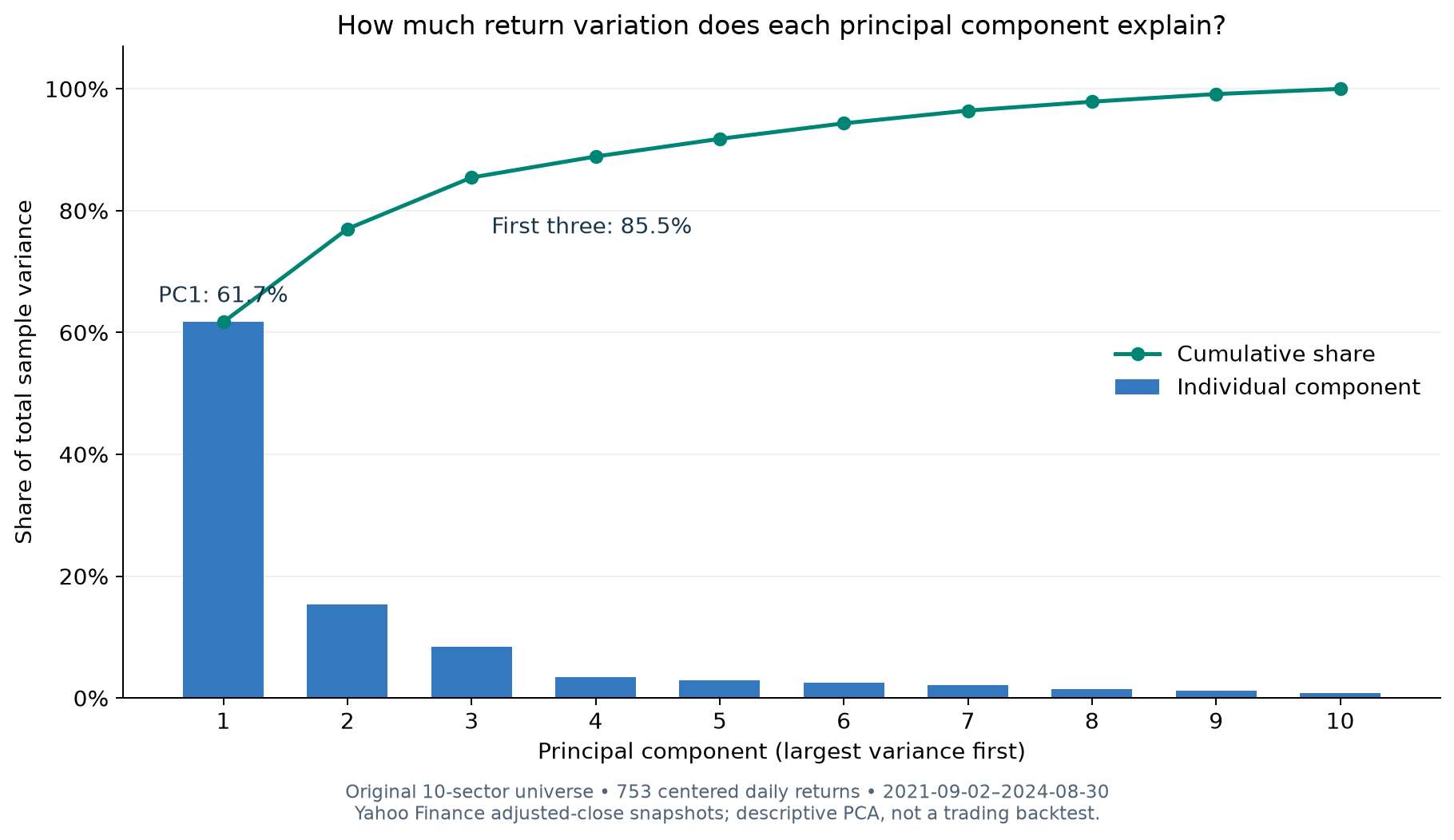
Figure 3. A fresh, centered calculation for the original ten-sector universe: XLB, XLC, XLE, XLF, XLI, XLK, XLP, XLU, XLV, and XLY. The window contains 753 daily returns from September 2, 2021 through August 30, 2024. The original figure used uncentered SVD; this replacement also numbers components from 1 and shows cumulative variance. Source: cached Yahoo Finance adjusted closes; plotting inputs and provenance accompany the figure in the repository.
The first component explains 61.7% of total sample variance. The first three explain 85.5%. That tells us the returns share substantial common structure. It says nothing by itself about expected returns, future benchmark tracking, or the best trading allocation.
There is a further distinction for a particular portfolio. For weights $w$,
\[\operatorname{Var}(Rw) =w^\top\widehat\Sigma w =\sum_i\lambda_i(v_i^\top w)^2.\]The exposure $v_i^\top w$ matters alongside the eigenvalue. A component explaining 61.7% of variance across the whole asset universe need not explain 61.7% of a chosen portfolio’s risk.
5. Where these ideas enter systematic investing
The decomposition supplies a representation of the data. An investment process still needs an objective, constraints, a trading schedule, and an evaluation method.
| Application | Role of SVD/PCA | What remains to be established |
|---|---|---|
| Risk diagnostics | Identify common return directions and measure portfolio exposures | Whether the directions are stable and economically interpretable |
| Covariance estimation | Model common covariance with a limited set of factors | Whether the restriction improves future risk estimates |
| Portfolio allocation | Supply the risk model for an optimizer | The objective, position limits, costs, and return tradeoffs |
| Hedging | Construct portfolios with limited exposure to selected components | Feasibility, turnover, estimation error, and omitted risks |
| Residual signals | Separate fitted common movements from residual returns | A separate predictive hypothesis; residuals need not mean-revert |
| Feature compression | Use component scores as inputs to a forecasting model | Predictive validation and fitting the transformation only on training data |
The implementation here covers risk diagnostics, covariance estimation, and minimum-variance allocation. The other rows describe possible extensions, rather than strategies tested by this repository.
A principal direction is not yet a portfolio rule
Consider two equally volatile assets with positive correlation. Their first component points roughly in the common long direction, while the second points along their relative spread. The leading component is the direction with the most variance under the PCA normalization. A lower-variance allocation is a different optimization problem.
Principal directions also have unit Euclidean norm, not necessarily weights summing to one. They may contain shorts or have a sum close to zero. Taking absolute values can destroy an intended hedge; dividing by the sum can create extreme exposures. The global sign ambiguity of an eigenvector is harmless, but changing the relative signs of its entries is not.
For this reason, I use PCA to estimate covariance and then solve a clearly specified allocation problem. I do not turn the absolute values of the first loading vector directly into the strategy.
Preserve risk outside the retained components
A pure truncated covariance estimate is
\[\Sigma_{\text{common}}=V_k\Lambda_kV_k^\top.\]It assigns zero variance to directions outside the retained subspace. An optimizer could exploit that assumption. Instead, the model retains a diagonal residual term:
\[D=\operatorname{diag}\!\left(\operatorname{diag} \left(\widehat\Sigma-\Sigma_{\text{common}}\right)\right), \qquad \widehat\Sigma_k=\Sigma_{\text{common}}+D.\]This preserves every asset’s sample variance and assumes residual cross-asset covariances are zero. The assumption can reduce estimation noise, but it can also discard genuine hedges. It is a modeling choice to test, even when the retained variance looks impressive.
The implemented allocation is
\[\min_w w^\top\widehat\Sigma_k w \quad\text{subject to}\quad \mathbf{1}^\top w=1,\qquad 0\leq w_i\leq0.30.\]This is a constrained minimum-variance portfolio. It has no expected-return forecast, and it does not optimize tracking error against SPY or AOM. Those would require different objectives.
6. Connect the equations to Python
The following example reproduces the descriptive ten-sector PCA window. Run it from the repository root after caching the data with the commands in the README.
1
2
3
4
5
6
7
8
9
10
11
12
13
14
15
16
17
18
19
20
21
22
23
24
25
26
27
28
29
30
31
from pathlib import Path

import numpy as np
import pandas as pd

from svd_portfolio.config import UNIVERSES, ResearchConfig
from svd_portfolio.data import load_prices, simple_returns

prices, _ = load_prices(UNIVERSES["us_equity"], ResearchConfig(), Path.cwd())
tickers = [ticker for ticker in UNIVERSES["us_equity"].tickers if ticker != "XLRE"]
sample_prices = prices.loc["2021-09-01":"2024-08-31", tickers]
sample_returns = simple_returns(sample_prices)

mean_returns = sample_returns.mean()
X = (sample_returns - mean_returns).to_numpy()
U, s, Vt = np.linalg.svd(X, full_matrices=False)
V = Vt.T

explained_variance = s**2 / np.sum(s**2)
scores = pd.DataFrame(
    U * s,
    index=sample_returns.index,
    columns=[f"PC{i + 1}" for i in range(len(s))],
)

k = 3
X_k = (U[:, :k] * s[:k]) @ Vt[:k, :]
np.testing.assert_allclose((U * s) @ Vt, X, atol=1e-12)
np.testing.assert_allclose(X @ V, scores.to_numpy(), atol=1e-12)
print(f"PC1: {explained_variance[0]:.1%}")
print(f"First {k}: {explained_variance[:k].sum():.1%}")
Vt contains the transposed asset directions, s contains their singular values, and U * s scales each column of U. The final two assertions connect the code to the reconstruction and score equations above. This fits one descriptive historical window; it is not a backtest.
The same window can illustrate covariance construction and the constrained optimization:
1
2
3
4
5
6
7
8
9
from svd_portfolio.models import minimum_variance, pca_covariance

fit = pca_covariance(sample_returns, n_components=3, space="covariance")
weights = pd.Series(
    minimum_variance(fit.covariance, cap=0.30),
    index=sample_returns.columns,
    name="Illustrative target weight",
)
print(weights.round(4))
The tickers remain attached to the weights, preventing a mismatch between returned column order and manually supplied labels. In the systematic experiment, this calculation is repeated using only the history available at each decision date.
7. Test whether the risk model helps
The empirical question is: does a PCA covariance model improve subsequent portfolio risk and risk forecasts relative to sample covariance and Ledoit–Wolf shrinkage, after costs?
I use eleven US sector ETFs, adding XLRE to the original ten, and the original twelve multi-asset ETFs. Equal weighting and capped inverse volatility provide simple allocation controls. The sample-covariance optimizer isolates the impact of regularization, while Ledoit–Wolf shrinkage provides a practical alternative. The empirical results of DeMiguel, Garlappi, and Uppal (2009) are a useful reason to retain simple controls rather than assume that optimization will outperform them.
The primary specification uses a 504-session training window, three components, and a 30% maximum target weight. On the first session of each month, the model uses information through the previous session, trades at the current close, and earns returns on the new positions from the following session. Existing positions earn the execution day’s return before the trade. Weights drift between monthly rebalances.
Costs are 5 basis points per dollar bought or sold, including entry. The accounting allows for the cash required to pay those costs. The implementation assumes fractional holdings and close execution, with no taxes or market-impact model.
The price history covers July 2018–August 2026. Evaluated portfolios begin in August 2020, and January 2025–August 2026 is the retrospective historical test. The March 2020 crash is in training, not in the evaluated portfolio history. This is not a genuinely untouched holdout, and the data are current-vintage adjusted closes rather than a point-in-time institutional archive.
The teaching chart in Figure 3 is kept separate: its three-year, ten-ETF fit explains the concept; no loading from that whole window is fed into the rolling backtest.
What the executed experiment shows
The primary outcome is net annualized volatility over 416 historical-test sessions. The table reports PCA minus Ledoit–Wolf in percentage points. Its pointwise 95% intervals use paired 21-session circular blocks and 2,000 bootstrap resamples.
| Universe | PCA volatility | Ledoit–Wolf volatility | Difference (pp) | 95% CI (pp) |
|---|---|---|---|---|
| US sector ETFs | 11.92% | 11.99% | -0.075 | [-0.224, +0.053] |
| Multi-asset ETFs | 3.14% | 3.21% | -0.068 | [-0.113, -0.020] |
- US sector ETFs: PCA has lower historical-test volatility in 4/10 declared specifications. Its mean QLIKE difference versus Ledoit–Wolf is -0.0049 (95% interval [-0.0869, +0.0404]).
- Multi-asset ETFs: PCA has lower historical-test volatility in 9/10 declared specifications. Its mean QLIKE difference versus Ledoit–Wolf is -0.0131 (95% interval [-0.0577, +0.0164]).
The sector interval includes zero, and several reasonable changes to the specification reverse the ranking. The multi-asset effect is small in absolute terms. Its PCA portfolio puts about 89% of the average historical-test target allocation in AGG, IAGG, and SHY. The low volatility must therefore be interpreted alongside its concentrated bond exposure and modest return.
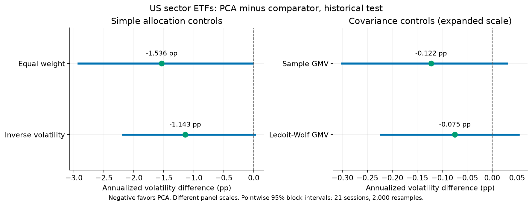
Figure 4. Sector results for January 2025–August 2026. Negative differences favor PCA. The covariance-control panel uses an explicitly expanded scale so the small primary effect is visible. Intervals are conditional on the realized strategy paths, rather than on repeated model selection.
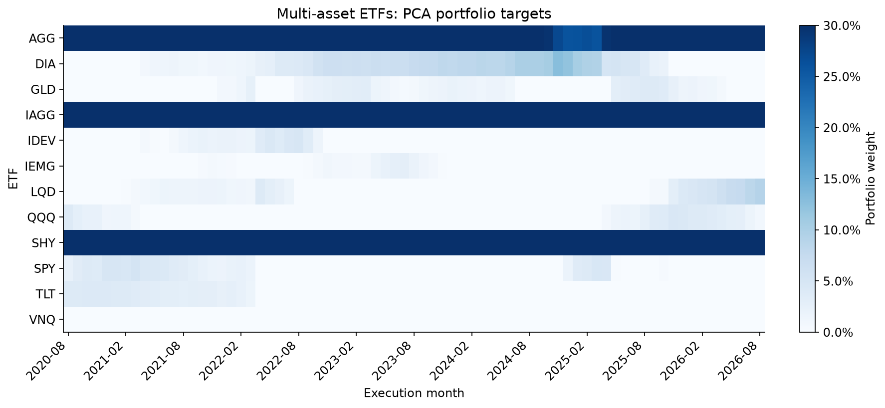
Figure 5. The multi-asset allocation is dominated by bond ETFs. Lower risk relative to equal weight or AOM needs to be read in that context; these are different economic exposures.
The sector PCA portfolio’s test-period net CAGR is about 10.96%; the multi-asset portfolio’s is about 4.49%. Lower volatility alone does not determine the best portfolio for an investor with a return objective. Full results are available in the results tables.
Forecast quality and robustness
A portfolio can become less volatile simply by choosing safer assets. To examine covariance forecasting separately, each model predicts the variance of the same daily equal-weight portfolio. The comparison uses a QLIKE loss against squared returns around the training mean. Patton (2011) discusses the importance of the loss function when evaluating volatility forecasts using noisy proxies.
The forecast-loss intervals include zero in both universes. The point estimates favor PCA, but the experiment does not establish better risk forecasts. Daily squared residuals are noisy, and the training-mean estimate adds another assumption.
I also report all ten declared specifications: the primary case, alternative factor counts, shorter lookbacks, correlation-space PCA, different costs, and different concentration limits.
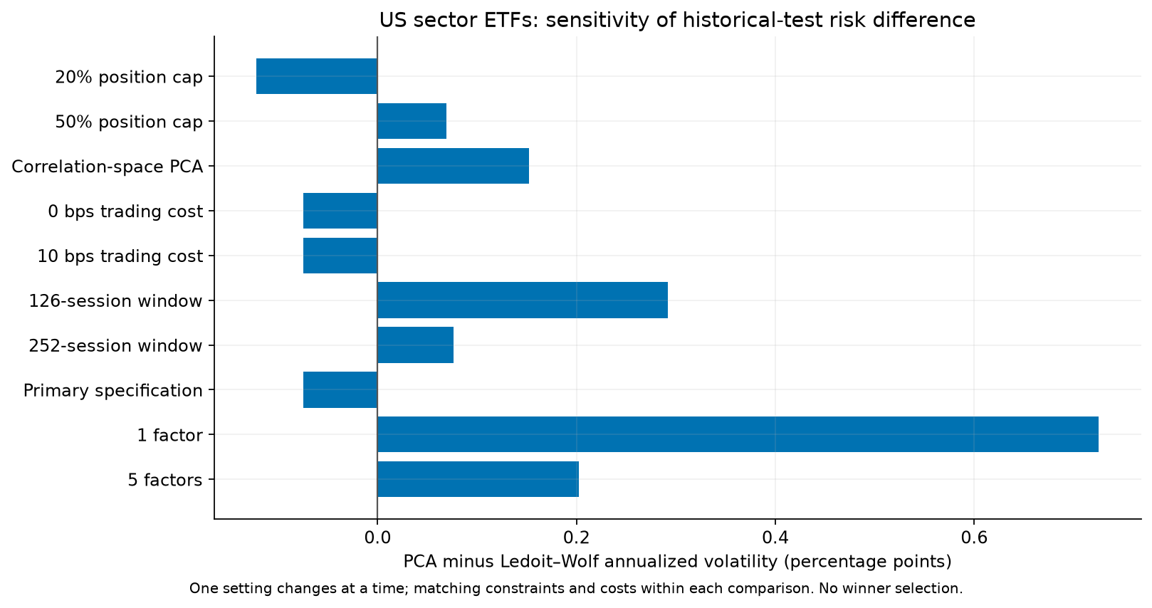
Figure 6. All specifications use the same test dates, with matching constraints and costs within each comparison. The variants share data and are not independent replications.
Choosing whichever variant looks best in this chart would create a new strategy requiring a new evaluation sample. The full protocol records these distinctions, the accounting rules, and the inference assumptions.
8. What SVD and PCA contribute
SVD decomposes a return matrix into directions and magnitudes. Applied to centered returns, it supplies the principal directions, score series, and explained-variance shares used in PCA. Truncating the decomposition gives an interpretable approximation of common return structure.
Using that structure in systematic investing requires more: an economic objective, a treatment of residual risk, implementable weights, and a test that respects information timing. This project makes that connection through a constrained portfolio risk model. The results show why a useful statistical representation can have only a small or unstable investment benefit.
The next research step is to freeze the specification before new observations arrive, add independently selected universes, and compare portfolios with more closely matched exposures. The sector notebook and multi-asset notebook provide the executed evidence and the code needed to examine those questions.
For the related regression problem, see factor exposures through SVD. There, the matrix columns are named factor returns; here they are asset returns. The same decomposition serves different economic questions.