
This post is about methodologies to measure private investment return (python code included). Reference for this post can be found in INSEAD case studies. Full python code can be found in my GitHub repo. And full case note from INSEAD can be found in this link. CASE_NOTE
Introduction
In the world of private equity (PE), measuring the performance of investments is not only crucial for assessing current financial health but also for strategic decision-making for future investments. This blog post explores why measuring private investment return is important, delves into the methodology, strengths, and weaknesses of five common methods (IRR, Modified IRR, LN PME, KS PME, Direct Alpha), and concludes with our recommendations for investors.
Major characteristics of private invetment is iliquid market and exotic structure. Methodologies introduced in this post will incorporate infrequent cash flow schedule which makes DCF based methodology difficult, and exotic investment structure which makes researchers to difficult to proxy private investment using public market data.
Why Measuring Private Investment Return is Important
Measuring the return on private investments provides investors with insights into the financial health and performance of their investments relative to the market. It helps in making informed decisions about where to allocate resources and how to strategize for future investments. By evaluating performance, investors can identify top-performing funds, assess fund managers’ effectiveness, and compare returns across different asset classes. This measurement is critical not only for maximizing returns but also for understanding the risks associated with private equity investments.
Full Code
You can see full code in here CODE
1
2
3
4
5
6
7
8
9
10
11
12
13
14
15
16
17
18
19
20
21
22
23
24
25
26
27
28
29
30
31
32
33
34
35
36
37
38
39
40
41
42
43
44
45
46
47
48
## Internal Rate of Return (IRR)
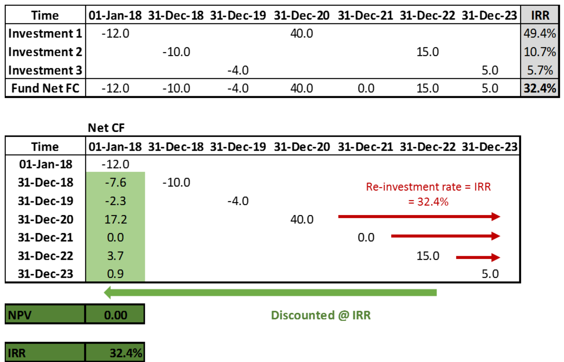
The IRR is a popular metric in the PE industry, representing the discount rate that brings the net present value (NPV) of a series of cash flows to zero. It considers the size and timing of the fund's cash flows. However, IRR assumes reinvested capital at the same rate, potentially overstating performance for early successful exits due to unrealistic reinvestment opportunities. Below figure illustrates the concept of IRR in excel format.
Below code is
```python
import os
import sys
from datetime import datetime
import numpy as np
import numpy_financial as npf
from scipy.optimize import newton
def days_between(d1, d2):
"""Calculate the number of days between two dates."""
d1 = datetime.strptime(d1, "%Y-%m-%d")
d2 = datetime.strptime(d2, "%Y-%m-%d")
return abs((d2 - d1).days)
def npv(rate, cashflows, days):
"""Calculate the net present value of cashflows at irregular intervals. (actual/360)"""
total_value = 0
for i, cashflow in enumerate(cashflows):
total_value += cashflow / ((1 + rate) ** (days[i] / 360))
return total_value
def irr(cashflows, dates):
"""Calculate the internal rate of return for irregular interval cashflows."""
# Calculate days between cashflows
start_date = dates[0]
days_diff = [days_between(start_date, date) for date in dates]
# Define a function to find the root
func = lambda r: npv(r, cashflows, days_diff)
# Use Newton's method to find the IRR
# Starting with an initial guess of 10%
# To guarantee convergence, please use bisection method
irr_result = newton(func, 0.1)
return irr_result
dates = ['2018-01-01', '2019-12-31', '2020-12-31']
cashflows = [-100, -20, 150]
irr_result = irr(cashflows, dates)
irr_result
Modified Internal Rate of Return (MIRR)
MIRR addresses the reinvestment assumption of IRR, assuming cash flows are reinvested at a more realistic return rate and taking into account the cost of uncalled capital. This method provides a more accurate measure of performance, adjusting for extreme performance cases in both directions. Below figure illustrates the concept of IRR in excel format. 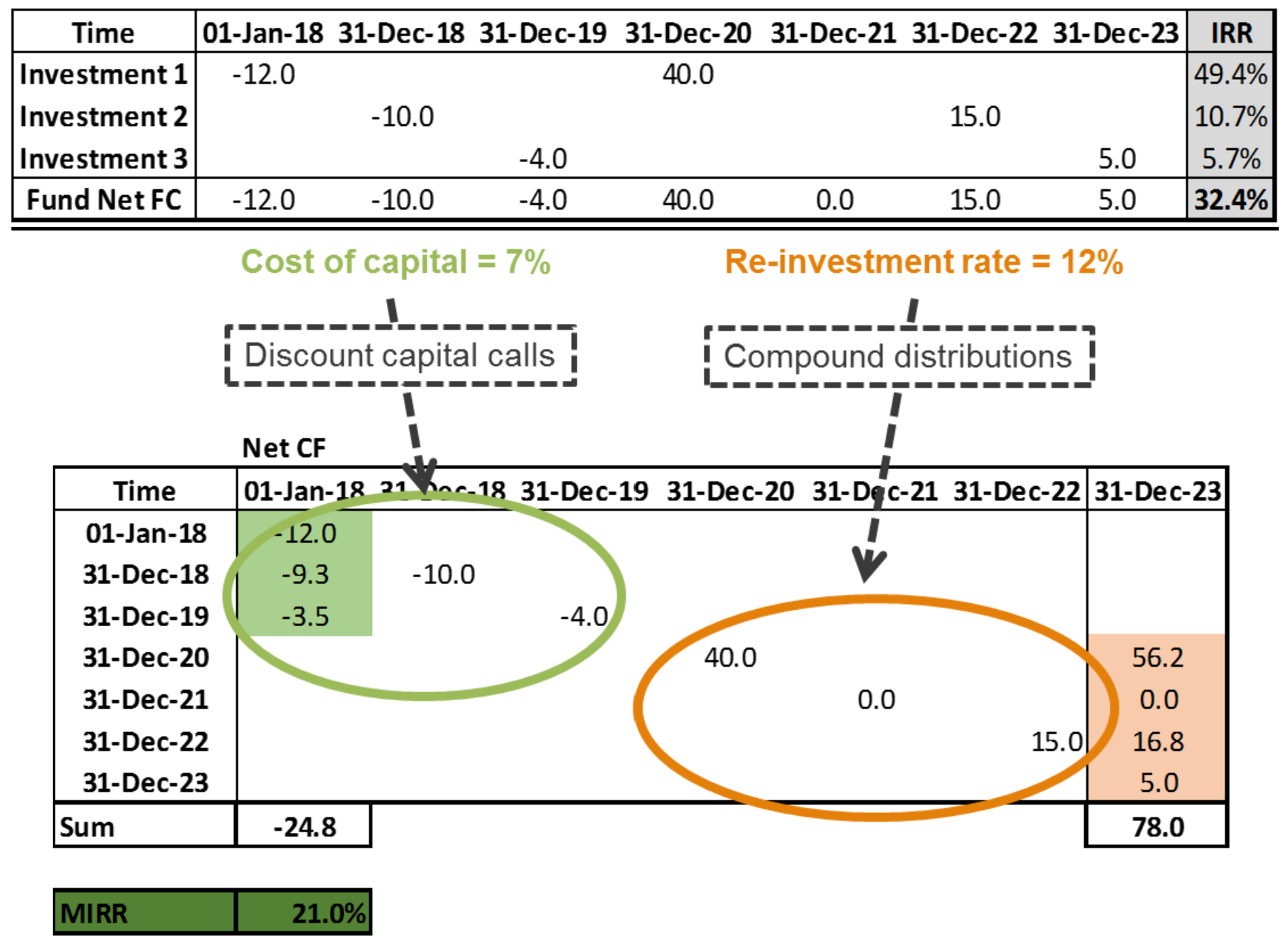
Below code is
1
2
3
4
5
6
7
8
9
10
11
12
13
14
15
16
17
18
19
20
21
22
23
24
25
26
27
28
29
30
31
32
33
34
35
36
37
38
39
40
41
42
43
44
45
46
47
48
49
50
import os
import sys
from datetime import datetime

import numpy as np
import numpy_financial as npf
from scipy.optimize import newton

def calculate_days(dates):
    """Calculate days between each date and the first date."""
    start_date = datetime.strptime(dates[0], "%Y-%m-%d")
    days = [(datetime.strptime(date, "%Y-%m-%d") - start_date).days for date in dates]
    return days

def objective_function(rate, pv_negative, fv_positive, days):
    """
    Objective function for the Newton method, calculating the NPV of modified cash flows at 'rate'.
    """
    npv = npf.npv(rate, [pv_negative] + [0]*(len(days)-2) + [fv_positive])
    return npv

def mirr_newton(cashflows, cost_of_capital, reinvestment_rate, dates):
    """
    Calculate MIRR using the Newton method, considering cost of capital and reinvestment rate.
    """
    days = calculate_days(dates)
    years = [day / 360 for day in days]  # Convert days to years for each cash flow

    # Separate positive and negative cash flows
    positive_cashflows = np.array(cashflows)
    positive_cashflows[positive_cashflows < 0] = 0
    negative_cashflows = np.array(cashflows)
    negative_cashflows[negative_cashflows > 0] = 0

    # Calculate the Present Value (PV) of negative cashflows at the financing rate
    pv_negative = npf.npv(cost_of_capital, negative_cashflows)

    # Calculate the Future Value (FV) of positive cashflows at the reinvestment rate
    fv_positive = npf.fv(reinvestment_rate, max(years), 0, -sum(positive_cashflows))

    # Use the Newton method to solve for MIRR
    mirr_result = newton(func=objective_function, x0=0.1, args=(pv_negative, fv_positive, days))

    return mirr_result

# Using the updated parameters for calculation
cost_of_capital = 0.08
reinvestment_rate = 0.12
dates = ['2018-01-01', '2019-12-31', '2020-12-31', '2021-12-31']
cashflows = [-100, -20, 50, 100]
Long Nickels Public Market Equivalent (LNPME)
LN PME compares a PE fund’s performance with a benchmark public index by creating a theoretical investment in the index using the fund’s cash flows. This method allows for direct comparison between PE and public market returns, albeit with potential shortcomings in cases of high distributions. Below figure illustrates the concept of IRR in excel format. 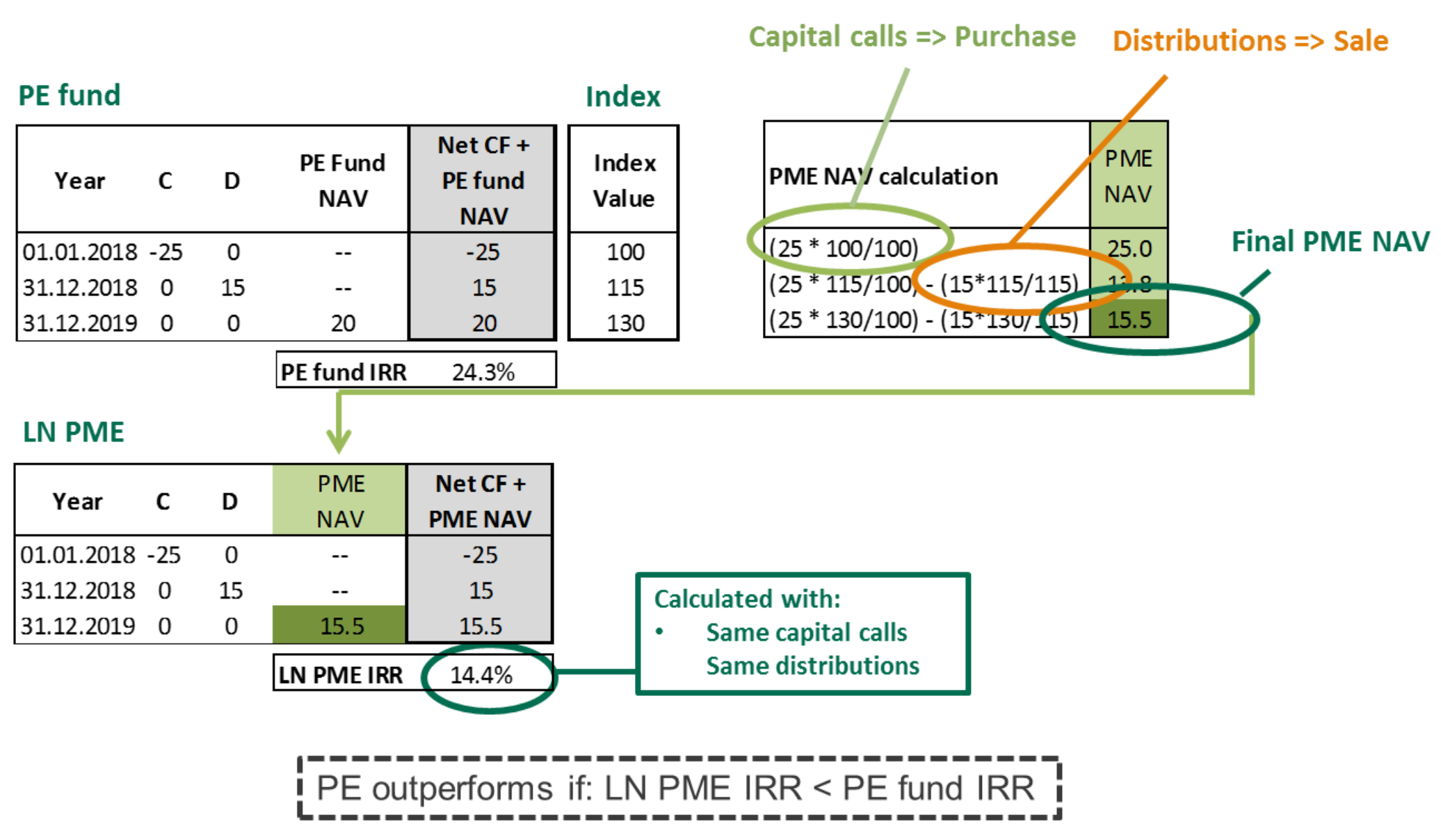
Below code is
1
2
3
4
5
6
7
8
9
10
11
12
13
14
15
16
17
18
19
20
21
22
23
24
25
26
27
28
29
30
31
32
33
34
35
36
37
38
39
40
41
42
43
import os
import sys
from datetime import datetime

import numpy as np
import numpy_financial as npf
from scipy.optimize import newton

def calculate_ln_pme(cf_dates, cf_schedule, index_values):

    PME_NAV_list = []
    PME_NAV_val = 0
    contribution, distrubution = 0,0
    for i in range(0, len(cf_dates)):
        if cf_schedule[i] < 0:
            contribution = contribution -(cf_schedule[i]/index_values[i])
        elif cf_schedule[i] > 0:
            distrubution = distrubution - (cf_schedule[i] / index_values[i])

        NAV_value = index_values[i] * (contribution + distrubution)
        PME_NAV_list.append(NAV_value)

    final_PME_NAV = PME_NAV_list[-1]

    # Final PME NAV calculation with the last NAV included
    adj_PME_NAV = cf_schedule
    adj_PME_NAV[-1] = final_PME_NAV

    # Calculate IRR of adjusted cash flows
    pme_irr = npf.irr(adj_PME_NAV)
    return final_PME_NAV, pme_irr

# Given data
cf_dates = ['2018-01-01', '2018-12-31', '2019-12-31']
cf_schedule = [-25, 15, 0] # Including the final NAV as a distribution
index_values = [100, 115, 130]

last_NAV = 20

# Calculate LN PME
final_pme_nav_value, ln_pme_irr_value = calculate_ln_pme(cf_dates, cf_schedule, index_values)

print(final_pme_nav_value, ln_pme_irr_value)
Kaplan Schoar Public Market Equivalent (KS PME)
KS PME measures the wealth multiple effect of investing in a PE fund versus an index, adjusting cash flows based on index performance. This method highlights the relative performance of a PE fund to the public market, though it overlooks cash flow timing. Below figure illustrates the concept of IRR in excel format. 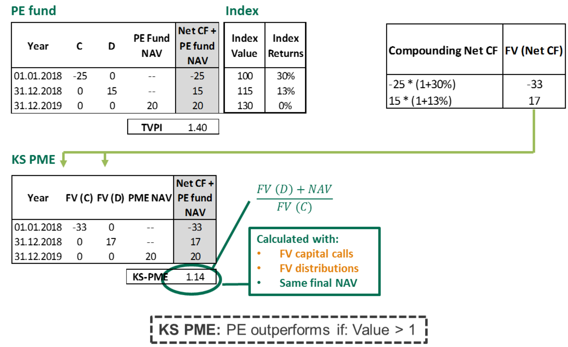
Below code is
1
2
3
4
5
6
7
8
9
10
11
12
13
14
15
16
17
18
19
20
21
22
23
24
25
26
27
28
29
30
31
32
33
34
35
36
37
38
39
40
41
42
43
44
45
46
47
import os
import sys
from datetime import datetime

import numpy as np
import numpy_financial as npf

def calculate_ks_pme(cf_dates, cf_schedule, index_values):

    PME_NAV_list = []
    PME_NAV_val = 0
    contribution, distrubution = 0,0


    index_return = []
    for i in range(len(index_values)):
        index_return.append((index_values[-1] / index_values[i]) - 1)

    adj_fv_list = []
    for i in range(len(cf_schedule)-1):
        adj_fv_list.append(cf_schedule[i] * (1 + index_return[i]))

    adj_fv_list.append(cf_schedule[-1])

    dist_nav = 0
    contribute = 0

    for i in range(len(adj_fv_list)):
        if adj_fv_list[i] < 0:
            contribute = contribute - adj_fv_list[i]
        else:
            dist_nav = dist_nav + adj_fv_list[i]


    return dist_nav / contribute

# Given data
cf_dates = ['2018-01-01', '2018-12-31', '2019-12-31']
cf_schedule = [-25, 15, 20] # Including the final NAV as a distribution
index_values = [100, 115, 130]

last_NAV = 20

# Calculate LN PME
ks_pme_irr = calculate_ks_pme(cf_dates, cf_schedule, index_values)

print(ks_pme_irr)
Direct Alpha
Direct Alpha quantifies the out/underperformance of a PE fund by calculating the IRR of compounded cash flows plus fund NAV. This method offers a precise rate of return of outperformance, addressing some of the limitations of PME methodologies. Below figure illustrates the concept of IRR in excel format. 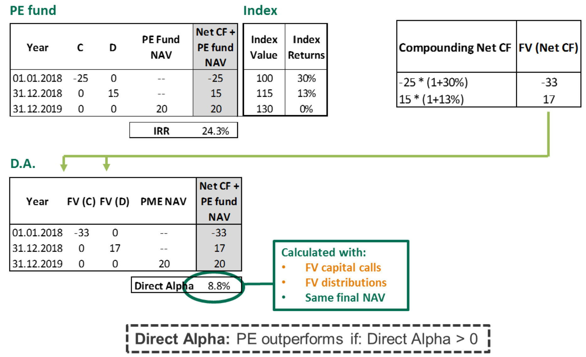
Below code is
1
2
3
4
5
6
7
8
9
10
11
12
13
14
15
16
17
18
19
20
21
22
23
24
25
26
27
28
29
30
31
32
33
34
35
36
37
38
39
import os
import sys
from datetime import datetime

import numpy as np
import numpy_financial as npf

def calculate_ks_pme(cf_dates, cf_schedule, index_values):

    PME_NAV_list = []
    PME_NAV_val = 0
    contribution, distrubution = 0,0


    index_return = []
    for i in range(len(index_values)):
        index_return.append((index_values[-1] / index_values[i]) - 1)

    adj_fv_list = []
    for i in range(len(cf_schedule)-1):
        adj_fv_list.append(cf_schedule[i] * (1 + index_return[i]))

    adj_fv_list.append(cf_schedule[-1])

    alpha = npf.irr(adj_fv_list)

    return alpha

# Given data
cf_dates = ['2018-01-01', '2018-12-31', '2019-12-31']
cf_schedule = [-25, 15, 20] # Including the final NAV as a distribution
index_values = [100, 115, 130]

last_NAV = 20

# Calculate LN PME
ks_pme_irr = calculate_ks_pme(cf_dates, cf_schedule, index_values)

print(ks_pme_irr)
Conclusion
Conclusion and Recommendations Investors in private equity face unique challenges in measuring and comparing returns due to the irregular timing and size of cash flows. While traditional metrics like IRR and MoM provide a starting point, more nuanced methodologies like MIRR, LN PME, KS PME, and Direct Alpha offer a more comprehensive view that accounts for the complexities of private equity investments. We recommend investors use a combination of these methods to gain a well-rounded understanding of their investment performance relative to the broader market.
As the PE market evolves, so too should the tools and methodologies we use to measure performance. It’s up to limited partners and investors to advocate for and adopt these more sophisticated measures, ensuring a deeper understanding and more effective management of their investments.
Understanding and accurately measuring investment returns is paramount in the dynamic landscape of private equity. By leveraging a combination of traditional and modern methodologies, investors can navigate this complex market with greater insight and precision.