
A vertical line placed neatly before a volatility spike can create a misleading impression of foresight. A segmentation algorithm may have needed the entire spike, and months of subsequent observations, to choose that line. The economically relevant question is therefore twofold: where did the distribution change, and when could the procedure have recognized it?
This distinction anchors the segmentation component of my renovated market-regime project. Historical segmentation describes periods with different return distributions. A separate synthetic experiment records alarms as observations arrive. It produces a revealing result: a large variance jump is detected reliably in the constructed paths, while the estimated break dates are systematically early.
The idea behind Gaussian segmentation
Suppose a time series can be divided into contiguous segments. Inside each segment, observations share a Gaussian mean and covariance; those parameters can change across boundaries. Unlike a mixture model, segmentation explicitly uses temporal contiguity. Similar distributions in two separated intervals do not automatically become the same recurring state.
Hallac, Nystrup, and Boyd’s Greedy Gaussian Segmentation formulates a regularized multivariate likelihood problem. Their algorithm alternates adding boundaries and adjusting existing ones, seeking a solution that cannot be improved by moving an individual breakpoint. The paper and its original implementation remain the methodological reference. The maintained project uses an independent, simpler univariate greedy splitter: it omits the original multivariate covariance regularization and breakpoint-refinement procedure. Its results should not be described as a full GGS replication.
For a segment containing $n=b-a$ scalar returns $x_a,\ldots,x_{b-1}$, the implemented estimates are
\[\hat\mu_{a:b}=\frac1n\sum_{t=a}^{b-1}x_t, \qquad \hat v_{a:b}=\frac1n\sum_{t=a}^{b-1}(x_t-\hat\mu_{a:b})^2.\]Away from the numerical floor, the following segment score equals twice the maximized Gaussian negative log-likelihood, up to constants:
\[C(a,b)=n\log\left(\max(\hat v_{a:b},10^{-10})\right).\]For a candidate boundary $k$, the improvement is
\[G(k)=C(a,b)-C(a,k)-C(k,b).\]A large positive gain means separate segment distributions explain the observed data better. The variance floor avoids an undefined logarithm; it is a numerical safeguard, with a negligible effect away from the floor. The algorithm selects the best admissible split, requires at least 40 observations on each side, and adds at most five boundaries, stopping when the best gain is below 20. These are declared settings, not parameters selected to reproduce famous crises.
What the historical boundaries mean
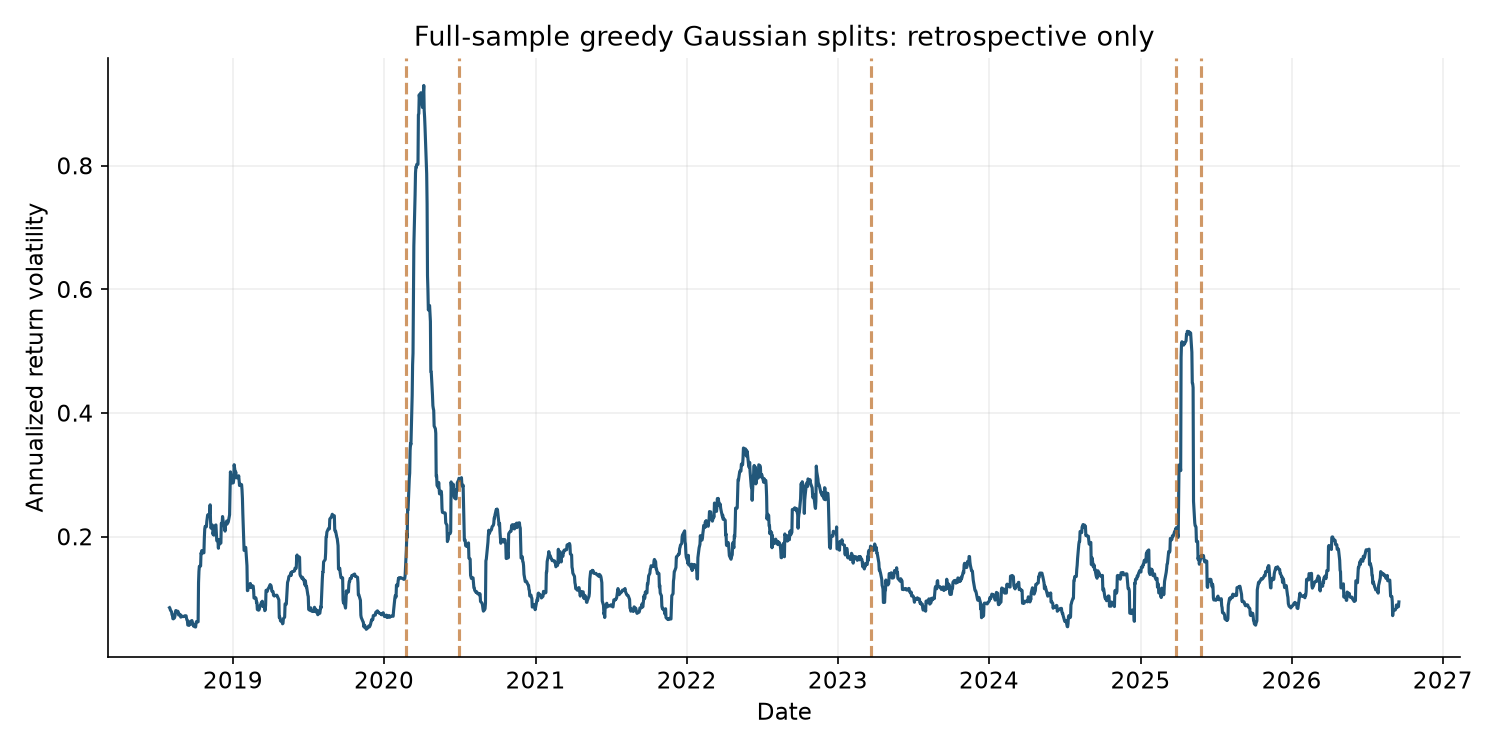
Original project figure. The line is 21-session realized equity volatility, annualized; 0.2 means 20%. Dashed boundaries are fitted using the complete return sample through 17 September 2026. The splitter operates on daily returns, not on the plotted rolling-volatility series.
The input contains 2,063 daily S&P 500 fund returns, beginning 3 July 2018. The saved interior boundaries are 24 February 2020, 30 June 2020, 23 March 2023, 28 March 2025, and 28 May 2025. Each is a full-sample estimate. For example, the February 2020 boundary must not be converted into a claim that the model issued a warning on that date.
The chart is useful for asking whether different parameter windows tell different risk stories, or whether a long fitted distribution is mixing very different scales. It cannot establish trading performance or economic causation. No boundary is validated as the start of a recession, a monetary-policy regime, or an investable signal. The complete boundary table also includes sample endpoints; these are not additional detected changes.
Detection needs a separate clock
The synthetic experiment constructs 400 independent standard-normal observations. In the change case, observations from index 200 onward are multiplied by three, giving a threefold volatility jump and ninefold variance jump. The no-change case retains constant variance. Fifty fixed seeds generate each case.
The procedure examines expanding prefixes every five observations, beginning with 80 observations, and stops at the first gain above 20. It saves both the alarm endpoint and the estimated breakpoint. They answer different questions and are never interchanged.
| Diagnostic | Observed result in the constructed paths |
|---|---|
| No-change paths with an alarm | 0 of 50 |
| Change paths detected after index 200 | 50 of 50 |
| Mean detection delay | 12.4 observations |
| Minimum–maximum detection delay | 5–30 observations |
| Mean estimated breakpoint | 169.26, versus true index 200 |
| Estimated breakpoints preceding the true break | 50 of 50 |
These values are calculated from the saved synthetic detection table. Zero observed null alarms in 50 paths is not proof of zero false-alarm probability. A large abrupt Gaussian variance change is also a favorable, narrowly defined test case; gradual changes, heavy tails, and multiple breaks remain untested here.
The localization error has an especially instructive mechanical explanation. With a 40-observation minimum on the right, a true boundary at 200 cannot even enter the candidate set until the endpoint reaches 240. Every observed alarm arrives earlier, between 205 and 230. The algorithm detects strong evidence of instability but must assign it to an earlier admissible boundary. A prompt alarm and an accurate change date are different achievements.
From description to a decision
An online detector would need a declared restart rule after each alarm, archived versions of every estimated boundary, and a fixed mapping from alarms to actions. Its usefulness would then depend on false alarms, delay, turnover, and subsequent losses. Those trading experiments have not been run for this splitter.
The project’s separate HMM forecast comparison reinforces this discipline: its late-segment loss difference against EWMA is +0.2539 [−0.1024, +0.8795], which does not establish added forecasting value. Good historical organization cannot substitute for that test. Explore the methods, executed notebook, and unrun next experiments for the complete distinction between description, detection, and prediction.