This post is about Regime Switching Model for financial market
What is Regime Switching Model
Financial market tend to show different behavior and pattern if market change their state. State is called “regime” in financial market. Easy example of regime switch is quantitative easying after COVID-19 outbreak in 2020, start of quantitative tightening in 2022. If we can determine what the regimes are, we can understand how a portfolio might react to various regime. This can enhance model’s predictability and reduce effort to build all-time effective killer model.
How to build regime switch model
Data-driven approach is letting historical data on assets and/or market risks delineate the regimes. An example of this approach is Greedy Gausian Segmentation algorithm. This algorithm segment multivariate time series via unsupervised learning method. GGS is heuristic method of complex dynamic programming which can reveal local optimum points.
Simple Math
For given K breakpoints, We want to regularize the covariance to avoid errors when there are more dimensions that samples in segment. So, we choolse $\beta$, $\mu$, $\sum$ to maximize the regularized log-likelihood.
$ (1) \phi(b, \mu, \sum) = \ell(b, \mu, \sum) - \lambda \sum_{i=1}^{K+1} Tr(\sum^{(i)})^{-1} = \sum_{i=1}^{K+1} (\ell^{(i)}(b_{i-1},b_i, mu^{(i)}, \sum^{(i)}) - \lambda Tr(\sum^{(i)})^{-1}) $
if $\lambda = 0$ this reduces to maximum likelihood estimation, but we will assume henceforth $ \lambda > 0$
If the breakpoints b are fixed, the regularized maximum likeluhood problem has simple analytical solutions. The optimal value of the ith segment mean is the empirical mean over the segment,
$ (2) \mu^{(i)} = \frac{b_i - b_{i-1}}{1} \sum_{t=b_{i-1}}^{b_{i-1}}x_t $ and the optimal value of the ith segment covariance is $ (3) \sum^{(i)} = S^{i} + \frac{b_i - b_{i-1}}{\lambda}I $
where $ S^{i} $ is the empirical covariance over the segment,
$ S^{i} = \frac{b_i - b_{i-1}}{1} \sum_{t=b_{i-1}}^{b_i -1}(x_t - \mu^{i}(x_t - \mu^{i}))^T $
Using these optimal values of the mean and covariance parameters, the regularized log-likelihood of (1) can be expressed in terms of b alone. $ (4) \phi(b) = C - \frac{1}{2} \sum_{i=1}^{K+1} \Biggl( (b_i - b_{i-1})log \, det \biggl( S^{i} + \frac{\lambda * I}{b_i - b_{i-1}} \biggr) - \lambda Tr \biggl(S^{i} + \frac{\lambda * I}{b_i - b_{i-1}}\biggr)^{-1} \Biggr) $
$ = C + \sum_{i=1}^{K+1}\psi(b_{i-1},b_i) $
where $C = -\frac{Tn}{2}(log(2 \pi) + 1) $ is constant that does not depend on b
We have reduced the regularized maximum likelihood estimation problem, for fixed value of K and $\lambda$, to the purely combinatorial problem.
Problem Statement in Math Form
$ (5) maximize -\frac{1}{2}\sum_{i=1}^{K+1} \Biggl( (b_i - b_{i-1}) log /, det \biggl( S^{i} + \frac{\lambda * I}{b_i - b_{i-1}} \biggr) - \lambda Tr \biggl (S^{i} + frac{\lambda*I}{b_i - b_{b-1}} \biggr) ^{(-1)} \Biggr) $ \
where the variable to be chosen is the collection of breakpoints $ b \,=\, (b_1,…,b_K)$.
These can take ${N-1 \choose K}$ possible values. And This is ultimate foumula we want to solve.
Simple Algorithm
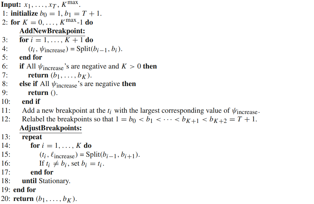
Building this idea requires two algorithm. First is to split time series into approximate intervals, and second is to choose split these breakpoints optimally.
Firt of all, to choose best break points, the function $(b_{i−1}, b_i)$ takes segment i and finds the t that maximizes $\psi(b_{i−1}, t) + \psi(t, b_i)$ over all values of t between $b_{i−1}$ and $b_i$ . The time t = $(b_{i−1}, b_i)$ is the optimal(highest) place to add a breakpoint between $b_{i−1}$ and $b_i$. The value of $\psi(b_{i−1}, t) + \psi(t, b_i) − \psi(b_{i−1}, b_i)$ is the increase in the objective if we add a new breakpoint at t. Due to the regularization term, it is possible for this maximum increase to be negative, which means that adding any breakpoint between $b_{i−1}$ and b_i actually decreases the objective.
Second, we use simple greedy method for finding good choices of K breakpoints, for K = 1, … , $K^{max}$, by alternating between adding a new breakpoints to the current set of breakpoints, and the adjusting the position of all breakpoints until the result shows optimal.
Why Greedy Gausian Segmentation Model for regime switch model
To be added
index data used
I used index data from major index maker. All index are available in ETF(Exchange Traded Fund) form and can be traded easily. Index data can be found from 1992 to 2021.
1
2
3
4
5
 Developed Market : MSCI world
 Emerging Market : MSCI Emerging
 Fixed Income : Bloomberg Barclays World AGG
 Risky Fixed Income : Bloomberg Barclays high yield bond
 Safety Fixed Income : Bloomberg Barclays Short-Term Treasury
Strategy Overview
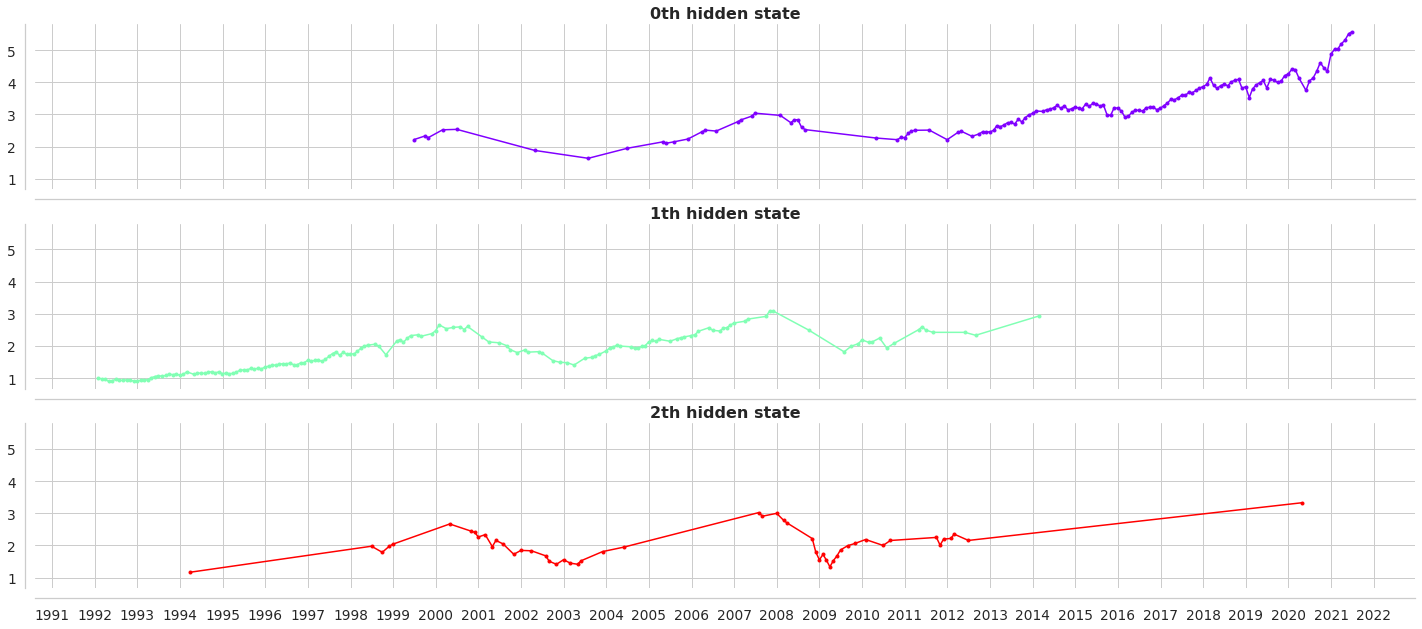
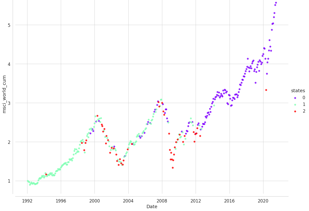
0th hidden state shows bull market regime. 1th hidden state shows sideways stock market regime. 2nd hidden state shows bear market regime.

1
2
3
4
5
6
7
8
Asset Class \ State           0th (mean / var)  1th (mean / var)  2nd (mean / var)
--------------------------    ----------------  ----------------  ----------------
mean Emerging Market          7.11433203e-03    0.01311532        -9.92782827e-03
vol  Emerging Market          2.01192349e-03    2.83001901e-03    1.16043600e-02
mean Risky Fixed Income       6.31190614e-03    0.01015012        -1.80401754e-03
vol  Risky Fixed Income       2.71058521e-04    8.79653083e-05    2.41111876e-03
mean Safety Fixed Income      1.24535026e-03    0.00452034        3.97258990e-03
vol  Safety Fixed Income      7.25365976e-06    2.01275656e-05    2.95434611e-05
Full Code
You can see full code in here CODE
Let’s code this idea
Mean variance strategy via python code. We used the networkx package to create Markov chain diagrams, and sklearn’s GaussianMixture to estimate historical regimes
1
2
3
4
5
6
7
8
9
10
11
12
13
14
15
16
17
18
19
20
21
22
23
24
25
26
27
28
29
30
31
32
33
34
35
36
37
38
model = mix.GaussianMixture(n_components=3,
                            covariance_type="full",
                            n_init=100,
                            random_state=8).fit(X)

# Predict the optimal sequence of internal hidden state
hidden_states = model.predict(X)

print("Means and vars of each hidden state")
for i in range(model.n_components):
    print("{0}th hidden state".format(i))
    print("mean = ", model.means_[i])
    print("var = ", np.diag(model.covariances_[i]))
    print()

sns.set(font_scale=1.25)
style_kwds = {'xtick.major.size': 3, 'ytick.major.size': 3,
              'legend.frameon': True}
sns.set_style('whitegrid', style_kwds)

fig, axs = plt.subplots(model.n_components, sharex=True, sharey=True, figsize=(20,9))
colors = cm.rainbow(np.linspace(0, 1, model.n_components))

for i, (ax, color) in enumerate(zip(axs, colors)):
    # Use fancy indexing to plot data in each state.
    mask = hidden_states == i
    ax.plot_date(select.index.values[mask],
                 select[target].values[mask],
                 ".-", c=color)
    ax.set_title("{0}th hidden state".format(i), fontsize=16, fontweight='demi')

    # Format the ticks.
    ax.xaxis.set_major_locator(YearLocator())
    ax.xaxis.set_minor_locator(MonthLocator())
    sns.despine(offset=10)
    # sns.despine(left=True, bottom=True)

plt.tight_layout()
Strategy Evaluation
To be added


