Black–Scholes–Merton in QuantLib: price, parity and the local hedge

A European option is a useful first QuantLib instrument because its price can be checked without another pricing engine. The payoff, financing assumptions and a normal-distribution formula give an independent reference. That makes it possible to ask a desk question: what exposure does this option add, and does the implementation measure that exposure consistently?

This example prices one European call at 9.319738, with spot delta 0.592749, under explicitly constructed assumptions. The direct formula, QuantLib analytic engine, put–call parity and finite-difference delta agree. These are numerical validation results, not observed option prices or evidence of a profitable hedge.

The contract behind the price

The valuation date is 15 September 2026. Spot and strike are both 100, maturity is exactly 365 days, the continuously compounded financing rate is 4%, the continuous dividend yield is 1%, and annual volatility is 20%. Actual/365 Fixed therefore makes the option horizon exactly one year. All inputs are illustrative.

The call pays $\max(S_T-K,0)$. With constant volatility and rates, the Black–Scholes–Merton value is

\[C=Se^{-qT}\Phi(d_1)-Ke^{-rT}\Phi(d_2),\qquad d_1=\frac{\log(S/K)+(r-q+\sigma^2/2)T}{\sigma\sqrt T},\qquad d_2=d_1-\sigma\sqrt T.\]

The dividend yield matters twice: it changes the forward level and discounts the spot term. Omitting it while retaining the same financing rate silently changes the economic contract. Volatility determines the dispersion of terminal values under the model; the convex payoff benefits from that dispersion.

A compact QuantLib implementation

Run this example from the maintained project’s root in its supported environment. The project’s valuation_date context restores QuantLib’s global evaluation date when the block finishes. The remaining construction follows the executed option notebook.

import QuantLib as ql
from research.pricing import DATE, valuation_date

with valuation_date():
    dc = ql.Actual365Fixed()
    process = ql.BlackScholesMertonProcess(
        ql.QuoteHandle(ql.SimpleQuote(100.0)),
        ql.YieldTermStructureHandle(ql.FlatForward(DATE, .01, dc)),
        ql.YieldTermStructureHandle(ql.FlatForward(DATE, .04, dc)),
        ql.BlackVolTermStructureHandle(
            ql.BlackConstantVol(DATE, ql.NullCalendar(), .20, dc)))
    call = ql.VanillaOption(
        ql.PlainVanillaPayoff(ql.Option.Call, 100.0),
        ql.EuropeanExercise(DATE + 365))
    call.setPricingEngine(ql.AnalyticEuropeanEngine(process))
    print(round(call.NPV(), 6), round(call.delta(), 6))
# 9.319738 0.592749

The process supplies spot, dividend, financing and volatility term structures. The option specifies the payoff and exercise rule; the engine chooses the valuation method. This separation lets a desk change a model assumption without changing the contract itself. The analytic engine source provides the implementation reference.

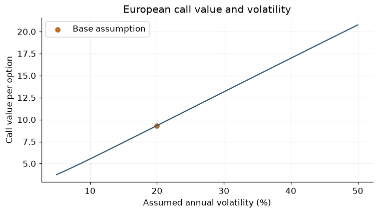Illustrative volatility sweep from the executed notebook. Spot, strike, rates, dividend yield and maturity remain fixed; no market volatility surface is fitted.

What the checks establish

The independent put value is 6.393699. Call minus put equals $Se^{-qT}-Ke^{-rT}$ within $10^{-10}$. This tests relative pricing and the dividend/financing signs. The separately calculated call also matches QuantLib within $10^{-10}$, while a symmetric spot perturbation of 0.001 matches its delta within $10^{-7}$.

Delta is the local change in option value per unit change in spot. At this point, shorting approximately 0.592749 underlying units offsets the instantaneous spot exposure of one long call under the model. That hedge changes as spot and time move. A one-percentage-point volatility change means 0.01 in decimal volatility units; confusing that with a change of 1 produces a hundredfold scaling error.

The volatility sweep shows how higher volatility increases the value of the convex payoff under the specified diffusion. It does not measure a realized volatility premium. Constant volatility, continuous dividends, European exercise and continuous hedging are material assumptions. Discrete dividends, exercise before expiry, jumps, transaction costs and smile dynamics require further modeling and evidence.

For rates applications, continue to caps and floors, where the option is attached to a floating coupon, or European swaptions, where the underlying is a forward swap and the annuity sets the price scale. Both examples retain explicit volatility units and independent parity checks.

Read the topic note · Explore the executed notebook · Browse all QuantLib desk examples