
A yield curve earns its place on a FICC desk by pricing dated cash flows consistently. The useful question is not how smoothly a line connects quoted rates. It is which instruments the curve reproduces, and what discount factors and forwards those instruments imply.
The maintained example builds a curve from ten illustrative OIS par quotes. Its one-year par quote is 3.80%, yet its continuously compounded zero rate is approximately 3.780411%. Both are correct for their stated conventions. Treating the par quote as a zero rate would change the instrument being priced.
Three objects with different meanings
A discount factor $D(0,t)$ is today’s value of one unit paid at date $t$. A continuously compounded zero rate summarizes that factor as
\[D(0,t)=e^{-z(t)t}.\]A simple forward rate for an accrual interval follows from two discount factors:
\[F(t_1,t_2)=\frac{D(0,t_1)/D(0,t_2)-1}{\tau(t_1,t_2)}.\]A par coupon rate instead makes a specified instrument’s initial value zero or its bond price par. It depends on the whole payment schedule. The year fraction used to report a zero rate need not equal the accrual convention used for a coupon or forward. That distinction is a contract choice, not rounding noise.
Build the instrument helpers first
The constructed inputs are dated 15 September 2026, cover 1–10 years, and use OIS helpers with a SOFR index. They are illustrative quotes, not a retrieved SOFR swap surface. The US GovernmentBond calendar and Modified Following payment adjustment are explicit. The primary curve interpolates log discount factors; zero rates are reported on Actual/365 Fixed and the annual simple forwards use Actual/360.
This compact example mirrors the discount-curve construction in the maintained pricing module. Run it from the project root. Calling a discount factor triggers QuantLib’s lazy bootstrap before helper residuals are requested.
1
2
3
4
5
6
7
8
9
10
11
12
13
14
15
16
17
18
19
import QuantLib as ql
from research.pricing import DATE, CAL, fixture, valuation_date

with valuation_date():
    quotes = fixture()
    helpers = [ql.OISRateHelper(
        0, ql.Period(int(row.years), ql.Years),
        float(row.ois_rate), ql.Sofr(),
        paymentConvention=ql.ModifiedFollowing,
        paymentCalendar=CAL) for row in quotes.itertuples()]
    curve = ql.PiecewiseLogLinearDiscount(
        DATE, helpers, ql.Actual365Fixed())
    curve.discount(curve.maxDate())
    errors = [h.impliedQuote() - float(q)
              for h, q in zip(helpers, quotes.ois_rate)]
    assert max(abs(e) for e in errors) < 1e-8
    one_year = CAL.advance(DATE, ql.Period(1, ql.Years))
    print(round(curve.discount(one_year), 6))
# 0.962902
A rate helper contains more than a number. It describes a quoted instrument, including its dates and conventions, whose theoretical quote the bootstrap must reproduce. QuantLib’s reference documentation is the API starting point; the project exposes the full helper configuration and pinned input file.
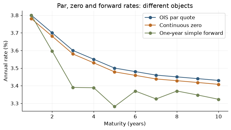 All three series use the same constructed quote set. They answer different pricing questions and are not competing estimates of one identical rate.
Read the curve before interpreting it
At ten years, the par quote is 3.43%, the continuous zero rate is 3.407709%, and the last annual simple forward is 3.322811%. That difference reflects instrument aggregation and conventions. Discount factors are positive throughout the covered range. The example does not require extrapolation beyond the available maturities.
The combined discount/projection calibration in the project has maximum quote error about $3.88\times10^{-14}$ in decimal rate units, below its declared $10^{-8}$ tolerance. Repricing inputs establishes internal consistency. Independent cash-flow calculations elsewhere in the project provide another validation layer; neither test converts constructed inputs into observations.
Curve inversion is a separate interpretation question. The curve-inversion notebook has an illustrative 10Y-minus-2Y zero spread of −27.3106 bp. A parallel zero-rate shift leaves that spread unchanged, while a shape shock changes it. This is a controlled identity check, not a recession forecast. A historical forecasting claim would require dated observations, a target, a decision-time information set and chronological evaluation.
The practical extension is projection versus discounting: once a floating index has its own projection curve, a single universal rate curve is no longer enough to describe both coupon forecasts and present values. The quotes and handles lab then shows how a stored instrument reacts to changed curve inputs.
Read the topic note · Explore the executed notebook · Browse all QuantLib desk examples