
A bond valuation should be explainable one payment at a time. If a model reports a clean price, the next questions are which cash flows remain, when they settle, how they accrue, and what curve discounts them. This post develops that workflow with a synthetic fixed-rate USD bond, retaining the bond-pricing purpose of the original article without implying that the example is an observed Treasury security.
Under the constructed primary curve, the bond is worth 103.195569 per 100 face on 15 September 2026. QuantLib and an independently reconstructed cash-flow sum agree. The useful result is the reconciliation: readers can follow the price back to a schedule and a set of assumptions.
Translate a ticket into dated payments
The bond has face value 100, a 4% annual coupon paid semiannually, an unadjusted schedule start of 15 March 2026 and maturity of 15 September 2033. Modified Following moves the schedule start to 16 March; the builder does not separately set an issue date. The example uses Actual/Actual ISMA accrual and the US GovernmentBond calendar. Settlement is zero days to align the valuation date, settlement date and independent present-value calculation.
For a settlement date $s$, the general cash-flow expression is
\[P_{dirty}(s)=\sum_{t_i>s}CF_i\frac{D(0,t_i)}{D(0,s)},\qquad P_{clean}(s)=P_{dirty}(s)-AI(s).\]Here $D(0,s)=1$ because settlement is the curve reference date. Reference-date and earlier payments are excluded consistently. For a different settlement convention, simply comparing a reference-date NPV with a settlement-date quoted price can create an apparent discrepancy even when both calculations are internally correct.
Accrued interest compensates for the contractual coupon accrual since the last coupon date. A clean price removes it for quotation; a dirty price includes it. Neither is a separate valuation theory.
Inspect the QuantLib instrument and the independent ledger
The following runnable excerpt uses the maintained project’s curve and bond builders. Run it from the project root. bond() constructs a FixedRateBond, attaches a DiscountingBondEngine, and separately reconstructs coupon amounts and principal from the schedule.
1
2
3
4
5
6
7
8
9
10
11
12
from research.pricing import valuation_date, curves, bond

with valuation_date():
    discount, _, _ = curves()
    instrument, flows = bond(discount)
    independent_pv = flows.pv.sum()
    assert abs(independent_pv - instrument.NPV()) < 1e-8
    assert abs(instrument.cleanPrice() + instrument.accruedAmount()
               - instrument.dirtyPrice()) < 1e-10
    print(round(instrument.cleanPrice(), 6))
    print(flows[["date", "amount", "discount", "pv"]].tail(2))
# Clean price: 103.195569
The notebook’s first calculation checks more than a second engine call: it builds the amounts from accrual fractions and multiplies them by dated discount factors. Inspect the last payment carefully. It contains both the final coupon and principal; forgetting either changes the price materially.
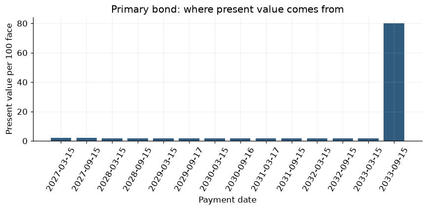 Present value per 100 face under the illustrative 15 September 2026 curve. The final payment combines 100 principal and a 2-unit coupon.
Why two valuation dates help
The primary valuation falls on a coupon date, so accrued interest is zero. That is useful for an initial reconciliation but insufficient to demonstrate the clean/dirty distinction. The notebook therefore includes a separate 15 October 2026 convention exercise, with a newly anchored flat continuous 3.5% curve.
| Exercise | Clean price | Accrued interest | Dirty price |
|---|---|---|---|
| September primary curve | 103.195569 | 0.000000 | 103.195569 |
| October flat-curve example | 102.835757 | 0.331492 | 103.167249 |
Both rows satisfy clean plus accrued equals dirty. The October row is not a holding-period return or a modeled path for the September curve: it changes the valuation date and deliberately supplies a separate curve. That separation prevents a convention illustration from being mistaken for an investment result.
The independent primary bond-PV discrepancy is approximately $2.84\times10^{-14}$ currency units. In a separate controlled comparison, changing coupon accrual to Actual/360 increases PV by 0.360369 per 100 face. The example therefore distinguishes negligible numerical error from a substantive change in the contract definition.
This bond has no credit, liquidity, tax or embedded-option spread. An observed Treasury CUSIP would require its actual schedule, settlement and quotation conventions, dated market inputs and appropriate source rights. A corporate bond would additionally require a defensible spread treatment. The present result establishes conditional numerical valuation, not a market fair-value claim.
Continue with bond risk and hedging to see why the maturity distribution in the chart matters for sensitivity, or with CDS hazard calibration to examine default-contingent cash flows separately.
Read the topic note · Explore the executed notebook · Browse all QuantLib desk examples