Financial Planning with Stochastic Programming

In the realm of financial planning, incorporating risk into investment decisions is paramount. This post explores a stochastic programming model aimed at optimizing investment strategies over a given time horizon to meet specific financial goals, such as funding a child’s college education.

Introduction

Financial decision-making often involves uncertainties that necessitate a probabilistic approach. Stochastic programming allows us to include randomness in our models, offering a more robust framework for financial planning. This model considers investment returns as random variables to optimize the allocation of initial wealth across different investments over multiple periods.

The Mathematical Model

The core of our model revolves around maximizing the expected utility of our final wealth, given the uncertainty of investment returns. Let’s define our variables and parameters:

• $b$: Initial wealth.
• $G$: Tuition goal after $Y$ years.
• $\xi(it)$: Return on investment $i$ in period $t$.
• $x(it)$: Amount invested in $i$ in period $t$.
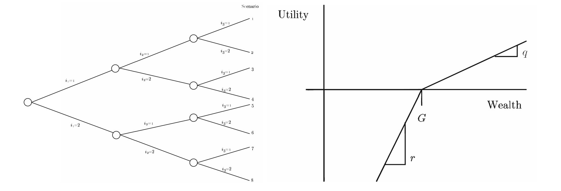
• $q$, $r$: Percent of the excess or shortfall, respectively, to the goal $G$.

Our objective is to maximize the expected utility:

\[\max Z = \sum_{s_1, \ldots, s_H} p(s_1, \ldots, s_H) \left( -r w(s_1, \ldots, s_H) + q y(s_1, \ldots, s_H) \right)\]

Subject to constraints ensuring that investments in each period adhere to the available wealth and achieve the goal $G$, while also considering investment returns as random variables:

\[\sum_{i} x(i1) = b\] \[\sum_{i} -\xi(it-1, s_1, \ldots, s_{t-1}) x(it-1, s_1, \ldots, s_{t-2}) + \sum_{i} x(it, s_1, \ldots, s_{t-1}) = 0\] \[\sum_{i} \xi(iH, s_1, \ldots, s_H) x(iH, s_1, \ldots, s_{H-1}) - y(s_1, \ldots, s_H) + w(s_1, \ldots, s_H) = G\]

In here, we assume the investors have risk-averse expected utilituy (concave curve, with utiligy gain =1, loss = 10, which means extremely risk-averse). Below diagram shows scenario trees generated by stochastic scenario and investors will take action in each stage to maximize their expected utility.

Using multi-stage scenario tress

In the stochastic programming model used, a multi-stage scenario tree represents the uncertainties in future investment returns, allowing for a dynamic investment strategy that can adjust based on realized outcomes.

The balance between preserving information and managing problem size is vital in constructing a scenario tree. For example, considering 100 scenarios over 50 stages results in an infeasibly large scenario space, highlighting the need for efficient scenario generation methods.

Evaluating scenerio tres

The quality of a scenario tree is crucial for the model’s performance. A good scenario tree should lead to sound decision-making, despite the inherent uncertainties of the future. Kaut and Wallace (2007) highlight two minimal requirements for a good scenario tree:

Stability: Multiple scenario trees should yield approximately the same optimal value of the objective function. Unbiasedness: The solution derived from the scenario-based problem should closely approximate the optimal solution of the original problem.

To enhance the scenario tress, this post use K-means (K=10) clusters to model the investment scenario.

## Insights and Analysis
Implementing this model for a scenario with two investment options (stocks and bonds) over 15 years, we observe that strategic reallocation based on past returns significantly improves the probability of meeting the financial goal. For instance, a stochastic model suggests a diversified investment strategy that dynamically adjusts, increasing the likelihood of achieving the tuition goal.

Full Code

You can see full code in here CODE

Let’s code this idea

import os
import sys

import numpy as np
import pandas as pd
import matplotlib.pyplot as plt

from sklearn.cluster import KMeans
import cvxpy as cp

# Use past 10 years historical data - ETFs used
spy = pd.read_csv('SPY.csv')
agg = pd.read_csv('AGG.csv')

# convert price data into daily yield data
spy_log_ret = np.log(spy['Adj Close'] / spy['Adj Close'].shift(1))
agg_log_ret = np.log(agg['Adj Close'] / agg['Adj Close'].shift(1))

# df_logret is daily log return of stock and bond
df_logret = pd.DataFrame({'stock' : spy_log_ret, 'bond' : agg_log_ret})
df_logret.loc[0, ['stock','bond']] = 0.0 

# set parameter
_mu = df_logret.mean() * 251 
_sigma = df_logret.cov() * 251
print("average annual stock return is ", round(_mu.iloc[0],4), " and bond return is ",round(_mu.iloc[1],4) )

mu = _mu.values.T
sigma = _sigma.values
print("stock vol is ", round(_sigma.iloc[0,0],4), " bond vol is ",round(_sigma.iloc[1,1],4), " cov is ",round(_sigma.iloc[0,1],4))

# generate stock and bond return scenario under gausian distribution
num_samples = 10000
stock, bond = np.random.multivariate_normal(mu, sigma, num_samples).T

plt.scatter(bond, stock)
plt.xlabel('bond return')
plt.ylabel('stock return')
plt.title("stock-bond return scenario using Monte Carlo simulation")
plt.xlim(-1,+1)
plt.ylim(-1,+1)
plt.show()

# cluster the performance for the simulated data to reduce dimensionality
num_clusters = 10
kmeans = KMeans(n_clusters=num_clusters).fit(np.transpose([bond, stock]))

# K-means clustering + PCA (mean-covariance matrix)
plt.scatter(bond, stock, c=kmeans.labels_)
plt.scatter(kmeans.cluster_centers_[:,0], kmeans.cluster_centers_[:,1], s=100, 
            color='white', edgecolors='black', linewidths=3)
plt.xlabel('bond return')
plt.ylabel('stock return')
plt.title('K-means + PCA to reduce dimensionality --> 10 scenarios')
plt.xlim(-1,+1)
plt.ylim(-1,+1)
plt.show()

print("Probability of each scenario")
prob = np.zeros(num_clusters)
scenarios = 1 + kmeans.cluster_centers_

for i in range(num_clusters):
    prob[i] = np.count_nonzero(kmeans.labels_==i)/num_samples
    print("cluster ", i, " : ", round(prob[i]*100,2), "%")
    print("stock return: ", round(scenarios[i][1]-1,4), " bond return is: ", round(scenarios[i][0]-1,4))


# building two-stage stochastic program considering utility
x_0 = cp.Variable(2)
y = cp.Variable(num_clusters)
w = cp.Variable(num_clusters)

q = 1
r = 10

init_amount = 100
goal_amount = 108

probability = cp.Problem(
    cp.Maximize(prob.T @ (q*y - r*w)),
    [
    sum(x_0) == init_amount,
    scenarios @ x_0 - y + w == goal_amount * np.ones(num_clusters),
    x_0 >= 0,
    y >= 0,
    w >= 0
    ]
)

probability.solve(solver=cp.ECOS)

expected_return = (goal_amount + np.dot(prob, y.value - w.value)) / init_amount - 1
print("optimal allocation for stock = ", round(x_0.value[0],2), " bond = ", round(x_0.value[1],2))
print("expected_retun is ", round(100* expected_return, 2),"%")

fig, ax = plt.subplots(1,1)
ax.bar(range(num_clusters), np.round(goal_amount+y.value,2), color='green', width=0.95)
ax.bar(range(num_clusters), goal_amount, color='red', width=0.95)
ax.bar(range(num_clusters), np.round(goal_amount-w.value,2), color='grey', width=0.95)
ax.set_ylim([0, 160])
ax.set_xlabel('scenarios')
ax.set_ylabel('final wealth')
plt.title('Investment return for each scenario')

Conclusion

Stochastic programming offers a powerful framework for financial planning, accommodating the inherent uncertainty in investment returns. By considering multiple scenarios and optimizing decisions accordingly, investors can significantly enhance their strategies to meet financial goals with higher confidence.