
A floating-rate coupon needs a forecast of its index fixing and a discount factor for its payment date. Those are different modeling jobs. A desk implementation should make that distinction explicit before interpreting a price difference as a market opportunity.
The example holds one seven-year payer swap’s coupon fixed and changes only its projection assumption. With the calibrated term-projection curve and OIS discounting, the swap starts at par. Replacing term projection with the OIS curve changes its value to −3.092940 per 100 notional. Both calculations are internally consistent with their specified inputs; the difference measures a controlled modeling choice.
Why two curves appear
Write $P^{proj}(t)$ for the projection curve’s discount-like factors. For a synthetic term-index accrual period,
\[L(t_a,t_b)=\frac{P^{proj}(t_a)/P^{proj}(t_b)-1}{\tau_{index}(t_a,t_b)}.\]The projected coupon is then notional times the forecast rate times the contract accrual, discounted using $D^{disc}(t_{pay})$. The projection factor supports a forecast calculation; it is not automatically the discount factor used to value every payment.
This distinction is encoded in QuantLib by connecting an index to its forwarding handle and a swap engine to its discount handle. Calibration helpers must also know the discounting assumption used to price their quoted instruments. Building two unrelated curves and connecting them only at the final pricing step would miss that dependency.
A deliberately transparent input set
The fixture supplies 1–10Y OIS par quotes and a term-swap strip exactly 50 bp above them. These are constructed teaching inputs dated 15 September 2026, not observed quotes or an estimate of a bank credit premium. The term index is explicitly named “Illustrative USD 3M”; it is not presented as current USD LIBOR.
The primary setup uses the US GovernmentBond calendar, Modified Following, Actual/360 coupon accrual and log-linear discount interpolation. The discount curve is bootstrapped first with OIS helpers. Term SwapRateHelper instruments then bootstrap the projection curve while discounting their cash flows with the OIS handle. The full constructor arguments are visible in the maintained pricing module.
The excerpt below runs from the project root and preserves the contractual coupon in the counterfactual. curves() returns both QuantLib term structures and their input-repricing residuals; swap() attaches the distinct projection and discount handles.
1
2
3
4
5
6
7
8
9
10
11
12
from research.pricing import valuation_date, curves, swap

with valuation_date():
    discount, projection, calibration = curves()
    par_swap, _, coupon = swap(discount, projection)
    ois_projection_swap, _, _ = swap(discount, discount, coupon)
    assert calibration.residual.abs().max() < 1e-8
    print(round(100 * coupon, 6))
    print(round(par_swap.NPV(), 6),
          round(ois_projection_swap.NPV(), 6))
# Fixed coupon: 3.959824 percent
# Dual-curve PV: approximately 0; OIS-only projection PV: -3.092940
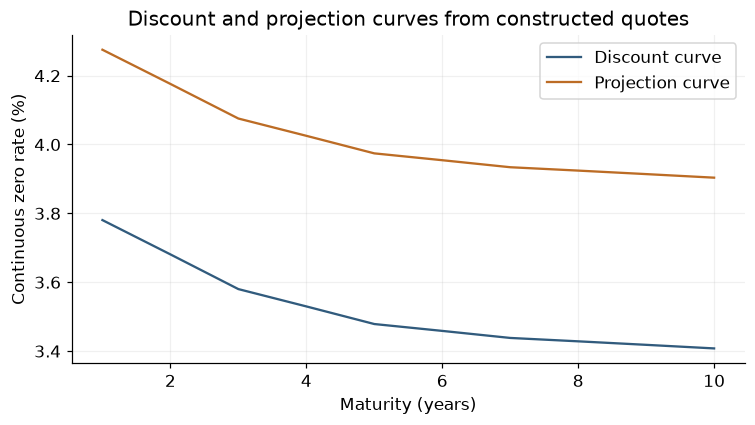 Two curves calibrated from the constructed quote strips. The valuation counterfactual substitutes the lower discount curve for projection while retaining the same fixed coupon, dates, notional and discounting.
Distinguish calibration from valuation evidence
The maximum residual across the two helper sets is approximately $3.88\times10^{-14}$ in decimal rate units, against a declared $10^{-8}$ tolerance. This confirms that each curve reproduces its input instrument quotes. It does not independently establish that the instrument conventions or quotes represent a live market.
The swap’s cash flows receive an additional independent reconciliation. Floating forecasts use index value and maturity dates, which can differ from coupon accrual dates after holiday adjustments. Multiplying a forward defined on one period by an incompatible year fraction creates a real convention difference. The maintained calculation therefore exposes both the index accrual and actual coupon accrual.
Interpolation has its own controlled comparison. Switching from log-linear discount interpolation to linear zero interpolation changes the bond PV by about −0.001539 per 100 and the frozen swap PV by +0.000278. These amounts are much smaller than the projection counterfactual here, but their relative size is specific to this fixture and these cash flows. Calibration at quoted instruments does not force agreement at every off-node date.
The exercise assumes a compatible collateral framework and has no live basis, futures convexity adjustment, fixing history or executable quote verification. It supports numerical understanding of projection and discounting, not a complete desk curve calibration. QuantLib’s documentation and the project source register identify the library references.
For a focused next step, the FRA lab isolates a single projected period and its start-settlement discounting. The quotes and handles lab explores live object updates; the IRS chapter carries the curves through full leg cash flows and annuity pricing.
Read the topic note · Explore the executed notebook · Browse all QuantLib desk examples