
A market regime model becomes useful when its state estimate improves a decision made with information available at the time. A convincing chart of past crises is an interesting description; the next question is whether those states improve a forecast.
My renovated regime research project tests this directly. Through 17 September 2026, a two-state hidden Markov model (HMM) does not establish better next-session equity risk forecasts than exponentially weighted volatility. Its late-segment mean loss difference is +0.2539, with a paired 95% block interval of [−0.1024, +0.8795]. Lower is better, so the point estimate favors the simpler baseline. This negative result is useful: it separates a model’s ability to organize history from evidence that its extra structure earns a place in a risk process.
What the hidden state contributes
A Gaussian mixture model (GMM) represents observations as draws from several distributions:
\[p(x_t)=\sum_{j=1}^{K}\pi_j\,\mathcal N(x_t;\mu_j,\Sigma_j).\]Components can capture different return scales, means, and combinations of asset behavior. The standard independent mixture has no transition mechanism: today’s component posterior classifies today’s observation, while its next-observation forecast uses the fitted mixture weights.
An HMM adds a transition matrix, with entry $A_{ij}=P(S_{t+1}=j\mid S_t=i)$. A persistent high-risk state can therefore affect tomorrow’s distribution. For filtered probabilities $\alpha_t(j)=P(S_t=j\mid x_{1:t})$, the forward update is
\[\alpha_t(j)\propto f_j(x_t)\sum_i\alpha_{t-1}(i)A_{ij}, \qquad p_{t+1\mid t}=\alpha_t A.\]The project normalizes this recursion in log space. A short known-parameter example checks it against exhaustive enumeration of hidden-state paths; changing future observations must leave previously archived forecasts unchanged. Full-sequence posterior and decoding routines require separate treatment because they can condition on later observations. See the hmmlearn API and the project’s implemented methods.
A small experiment with an explicit clock
The inputs are daily adjusted closes for an S&P 500 fund (SPY) and a long-maturity Treasury fund (TLT), from July 2018 through 17 September 2026. The first supplies the equity risk target; the second may distinguish equity stress from joint stock-and-bond shocks. The audited panel has 2,064 price dates and 2,063 return dates, with no missing sessions filled.
At each monthly refit, the preceding 504 returns, including that day’s close, determine scaling and model parameters. Both Gaussian models use two states and diagonal covariance matrices. States are ordered by their fitted equity second moment; “high risk” is a numerical description, with no claim that the state identifies a recession. The HMM updates its filtered belief between refits.
The forecast is a probability-weighted second moment in original return units:
\[v_{t+1\mid t}=\sum_jp_{t+1\mid t}(j)(\sigma_j^2+\mu_j^2).\]Every model faces the same target, next-session squared equity return, and the same loss:
\[L(v,r^2)=\log v+\frac{r^2}{v},\qquad v\ge10^{-8}.\]This penalizes an inadequate risk forecast when a large move occurs. Its level is not a return percentage; negative values are normal. A daily squared return is also a noisy proxy for conditional risk, rather than an observation of latent volatility. EWMA, with decay 0.94, and a trailing single-state second moment provide simple controls.
What the comparison says
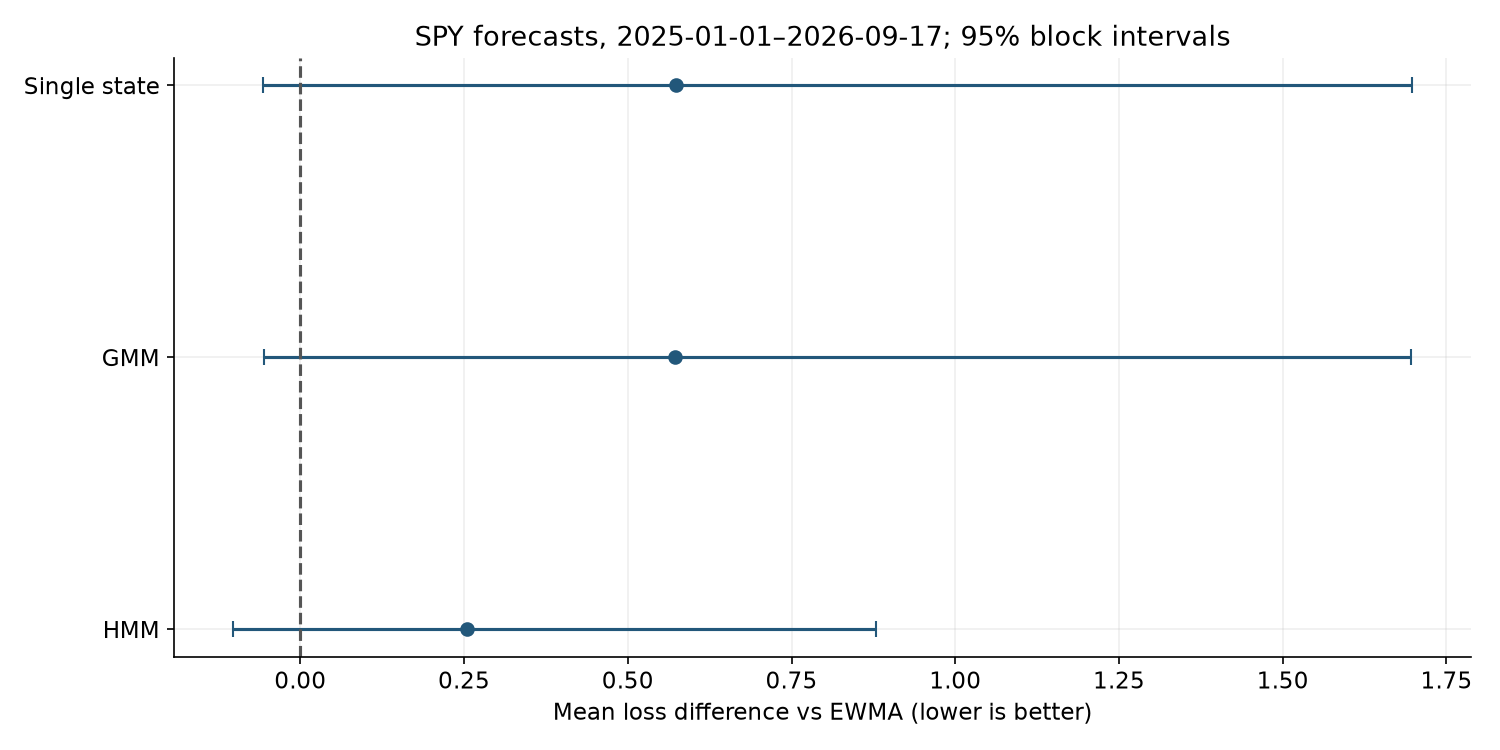
Original project figure. Dots show average loss differences from EWMA; bars are paired 95% intervals using 21-session circular blocks and 2,000 resamples. The HMM comparison is primary; the others are exploratory.
The primary late segment contains 428 matched forecasts. The ratio of total realized squared returns to total predicted second moments is 1.302 for HMM and 0.989 for EWMA: HMM understates aggregate risk in this segment. The wider post-warmup sample contains 1,538 forecasts, with an exploratory HMM-minus-EWMA difference of +0.1191 [0.0047, 0.2982] under the same block length. That comparison also favors EWMA.
Changing the state count, seed, covariance-floor setting, or feature set does not produce a favorable primary-direction point estimate. These dependent sensitivity checks cannot be counted as independent confirmations. The primary run has 74 refits and no failed HMM fits; the three-state variant has one failure and uses the declared EWMA fallback. The result tables retain every comparison.
Why the historical picture can look better
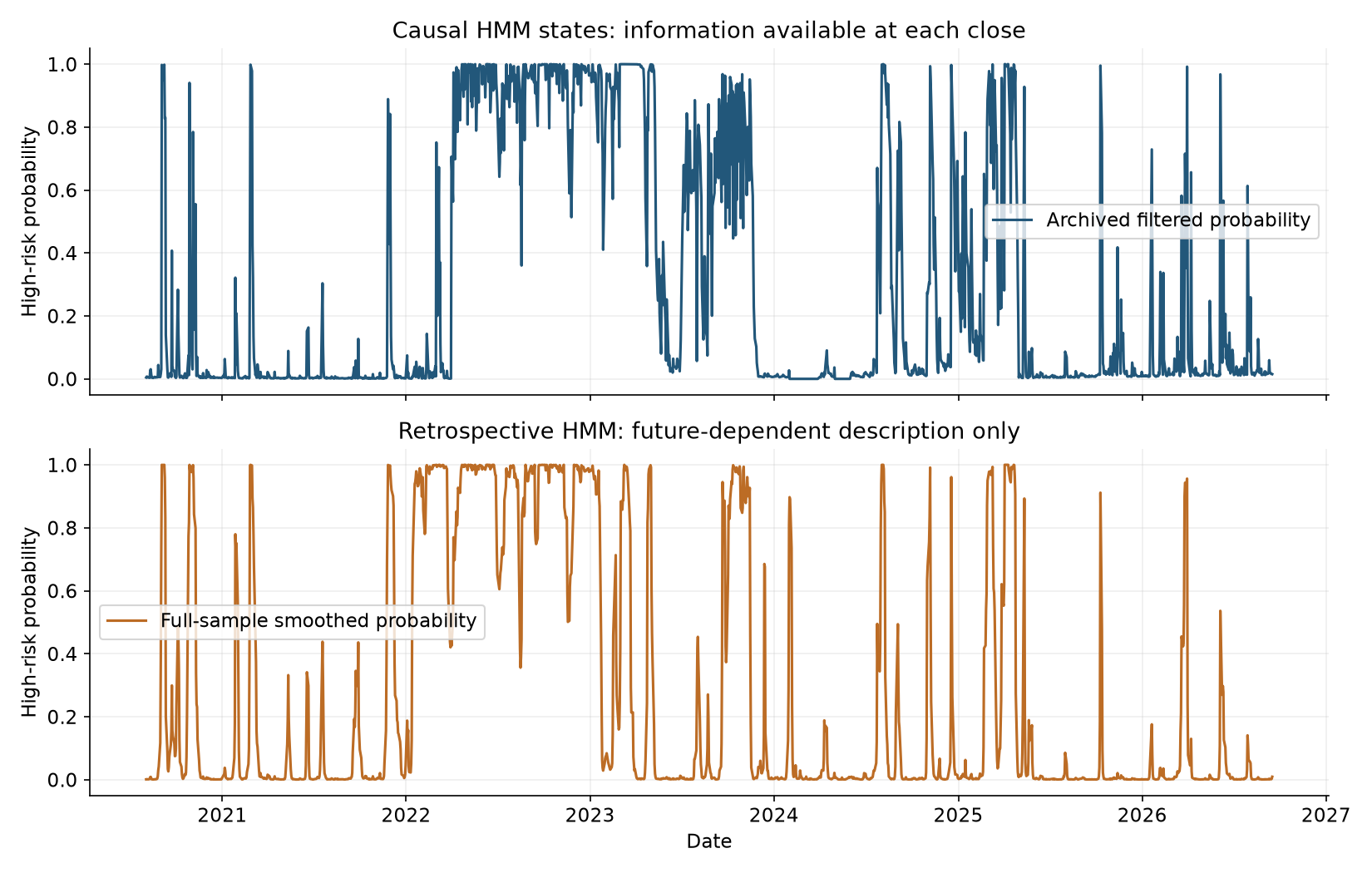
The upper panel uses each date’s available information. The lower panel fits and smooths with the full sample. Their difference combines parameter re-estimation and future conditioning; it does not isolate smoothing alone.
Thresholding each probability at 0.5 yields 15.28% disagreement between these historical descriptions. The retrospective chart remains useful for interpretation, but substituting its labels into a backtest changes the information set.
A supporting overlay maps high-risk probability $p$ to equity weight $1-0.75p$. It executes one close after the signal and first earns the following session’s return, charges 5 basis points per bought or sold dollar, and assumes zero cash interest. Its late-segment CAGR is 14.15%, versus 11.22% for a static 62.5% equity position. However, its average equity weight is 88.66%, versus 62.5% for the static control, and volatility is higher. That return difference does not establish timing skill; the paired mean-return/volatility difference interval against the static control includes zero.
The study is retrospective, uses revised vendor histories, and includes familiar market episodes. Its late segment is not an untouched holdout. The next useful experiment is a predeclared volatility-only model on genuinely new observations. The executed notebook, protocol, and source record make the present evidence inspectable.