
Maximum diversification and minimum variance optimize different ideas of risk. Minimum variance seeks the least volatile feasible portfolio. Maximum diversification asks how much risk is removed by combining the individual exposures. The distinction matters when a low-volatility asset can dominate a minimum-variance allocation without providing much breadth.
In the constructed example here, maximum diversification achieves a diversification ratio of 1.5419, compared with 1.4220 for minimum variance. Its annual volatility is nevertheless higher: 7.52% versus 6.94%. Neither outcome is contradictory. Each allocation does what its objective asks under the supplied covariance.
Define the risk reduction being optimized
Let $\sigma_i=\sqrt{\Sigma_{ii}}$ be individual asset volatility, and let $w$ be long-only weights summing to one. The diversification ratio is
\[DR(w)=\frac{w^\top\sigma}{\sqrt{w^\top\Sigma w}}.\]The numerator adds the weighted standalone volatilities. The denominator measures volatility after accounting for how the positions move together. Both use the same horizon, so the ratio is dimensionless.
If every exposure is perfectly positively correlated, a long-only combination has ratio one. For independent, equally volatile assets, equal weighting produces $DR=\sqrt N$. These limiting cases make the interpretation concrete: combining distinct risks can reduce aggregate variability relative to the sum of their individual contributions.
The objective does not contain expected returns. It also does not directly minimize losses in a tail scenario, drawdown, capital concentration or turnover. Those outcomes require separate inspection. The methodological paper develops the ratio-based construction; this article studies a bounded numerical example.
Compare objectives on exactly the same inputs
The executed notebook supplies three fictional assets with annual volatilities of 18%, 8% and 12%, labeled equities, long bonds and a diversifier. Their pairwise correlations are 0.20, 0.05 and 0.15. No observed prices or estimated mean returns enter the illustration.
Four long-only, fully invested rules use the same covariance:
| Rule | Diversification ratio | Annual volatility | Capital concentration, $\sum_iw_i^2$ |
|---|---|---|---|
| Maximum diversification | 1.541882 | 7.5213% | 0.355918 |
| Minimum variance | 1.422024 | 6.9366% | 0.506015 |
| Inverse volatility | 1.538968 | 7.3870% | 0.368421 |
| Equal risk contribution | 1.540785 | 7.4323% | 0.363163 |
Maximum diversification has the highest ratio by construction, while minimum variance has the lowest volatility. The small difference between maximum diversification and inverse volatility is also relevant: a numerical improvement in the targeted ratio need not justify a much more elaborate empirical decision rule.
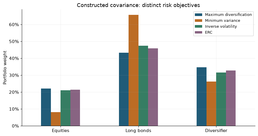
Constructed single-period allocation. The chart compares capital budgets under identical inputs and constraints, without leverage, historical returns or transaction costs.
Minimum variance allocates 65.61% to the least volatile asset, long bonds. Maximum diversification lowers that weight to 43.23%, while assigning 22.10% to equities and 34.67% to the diversifier. Its additional exposure to individually volatile assets increases total volatility but improves the ratio it was designed to maximize.
ERC pursues another objective: equal contributions to total portfolio risk. These rules can agree under special symmetric assumptions, but their names should not obscure their different economic jobs.
Check the numerical answer independently
When the unconstrained direction produces nonnegative weights, the interior maximum-diversification solution is proportional to
\[w\propto\Sigma^{-1}\sigma.\]The notebook checks that this direction is feasible in the constructed example and agrees with the constrained numerical solution. It independently verifies the equal-volatility, independent-asset limit and the perfectly correlated limit, along with every portfolio’s budget.
If the interior expression produces prohibited short positions, clipping and renormalizing it does not generally solve the constrained problem. The constraints need to enter the optimization itself. Nearly singular covariance and small changes in estimated correlations can also change the solution materially.
A robust empirical question
A high estimated ratio is a property of the estimated covariance. If correlations rise during a common shock, the diversification expected at the decision date can disappear. A strategy may also concentrate in several assets carrying the same economic risk even while their recent return correlations look modest.
The factor-risk chapter investigates that distinction. The estimation-risk laboratory shows how input perturbations and a changed correlation environment affect allocation. Expected-shortfall allocation changes the target to scenario tail losses and makes omitted scenarios visible.
The completed historical ETF study keeps a bounded primary family rather than adding maximum diversification as another contender after inspecting outcomes. A future historical comparison should declare its covariance estimator, lookback, constraints, execution schedule, costs and incremental endpoint in advance. Equal weight, inverse volatility and an appropriate risk control would help determine whether the extra estimation earns its complexity.
Continue with the detailed research note, worked notebook, and allocation research collection. The current evidence establishes the objective’s mechanics and its limits, without implying an empirical performance advantage.