
A portfolio optimizer translates beliefs into positions. It can make that translation precisely while the beliefs themselves remain uncertain. Mean–variance allocation is useful because it exposes the tradeoff: how much expected return justifies additional portfolio risk, and how strongly does the chosen answer depend on an estimated input?
The constructed study here makes the sensitivity visible. Raising one asset’s assumed annual return from 8% to 9%, while leaving covariance and constraints unchanged, moves its allocation from 45.96% to 56.05%. The additional ten percentage points of capital come from a one-percentage-point change in a forecast. That is a reason to investigate the forecast’s uncertainty before celebrating the optimizer’s solution.
The objective comes before the frontier
For weights $w$, expected simple returns $\mu$, and return covariance $\Sigma$, portfolio expected return is $w^\top\mu$ and variance is $w^\top\Sigma w$. All inputs must refer to compatible horizons and units.
One version of the allocation problem specifies a target expected return $m$:
\[\min_w w^\top\Sigma w\quad\text{subject to}\quad w^\top\mu=m,\quad\mathbf1^\top w=1,\quad w\geq0.\]This study permits neither short positions nor borrowing. Solving at a sequence of attainable return targets traces the long-only frontier. Its efficient portion begins at the global minimum-variance portfolio: an allocation below that point’s expected return can be dominated by another feasible mix with at least as much estimated return and no greater variance.
A different formulation chooses a risk penalty $\lambda$ and maximizes
\[w^\top\mu-\frac{\lambda}{2}w^\top\Sigma w.\]The choice of $\lambda$ is an economic preference. It is not automatically a maximum-Sharpe objective. Nor is $\lambda^{-1}\Sigma^{-1}\mu$ the general solution once a fully invested budget, long-only restrictions or other constraints enter the problem.
Read the frontier as an assumption map
The executed notebook supplies three fictional assets:
| Exposure | Assumed annual return | Assumed annual volatility |
|---|---|---|
| Growth asset | 8.0% | 18.0% |
| Intermediate bonds | 4.5% | 8.0% |
| Short bonds | 3.0% | 2.5% |
Their correlations are 0.20 for growth/intermediate bonds, 0.10 for growth/short bonds, and 0.35 for the two bond exposures. The resulting covariance is positive definite.
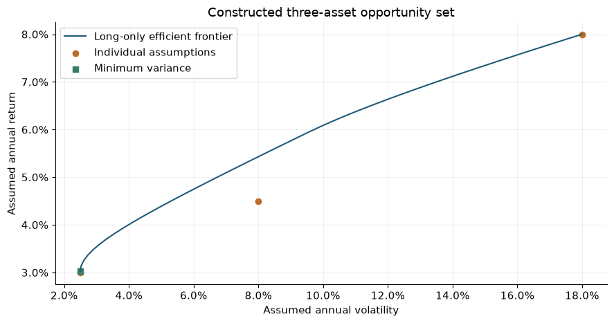
Constructed annual return and volatility assumptions. The curve describes feasible modeled portfolios; it is not a historical or forecast performance curve.
The minimum-variance solution holds 99.46% short bonds and 0.54% growth assets. At an expected return near 4.72%, the portfolio uses all three exposures. At the 8% endpoint, it holds the growth asset alone. Diversification is valuable within the supplied opportunity set, but the highest feasible return target ultimately removes it.
A small forecast change, a material trade
Holding the risk penalty at $\lambda=3$, the notebook changes only the growth asset’s expected return. The original allocation is 45.96% growth and 54.04% intermediate bonds. With the higher forecast it becomes 56.05% and 43.95%; short bonds receive zero in both cases.
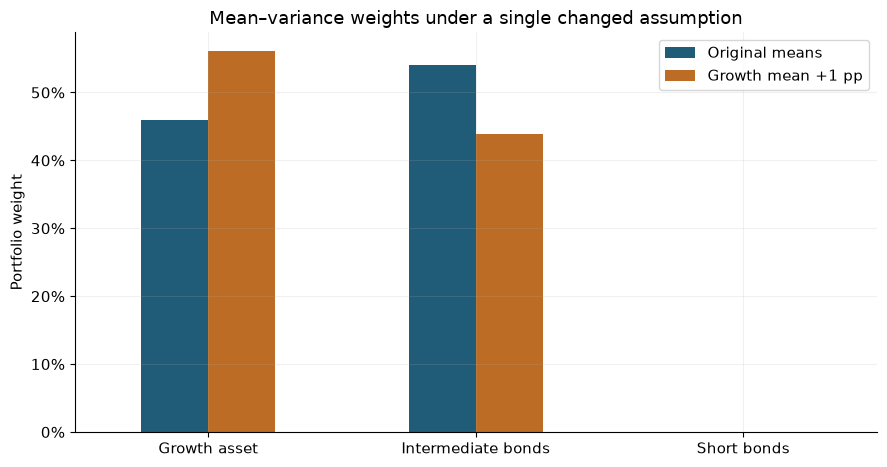
Controlled input perturbation. Covariance, risk penalty and long-only budget remain fixed.
This example isolates the response to a mean estimate. It does not prove that a ten-point weight change is always excessive. It asks what evidence supports treating the two forecasts as materially different. Repeatedly optimizing noisy sample means can produce trades that look purposeful while reflecting estimation error.
The notebook checks every budget and target-return constraint. An independent diagonal-covariance exercise compares the numerical minimum-variance solution with weights proportional to inverse variance. Solver correctness and forecast credibility are evaluated separately.
Building a more defensible decision
A robust research design limits how much uncertain estimates can change capital allocation. Constraints can restrict concentration; covariance shrinkage can stabilize risk estimates; a prior can temper noisy return views. Each introduces assumptions that deserve inspection. None creates information absent from the original data.
Black–Litterman allocation extends this question by making view confidence explicit. Expected-shortfall allocation changes the loss objective and reveals sensitivity to omitted tail scenarios. The estimation-risk laboratory compares fixed construction rules under perturbed inputs and a changed correlation environment.
These mechanisms remain separate from the project’s bounded historical ETF study, which does not add a new competition over return forecasts after inspecting its results. A future mean–variance test needs a declared forecast, training window, benchmark, timing and cost rule before evaluation.
For the theoretical context, see Markowitz’s Nobel lecture. Continue with the research note, worked notebook, and full allocation collection.