
An allocation can maximize estimated long-run growth and still be too large for the opportunity that actually exists. Kelly’s criterion makes this tension unusually clear: the fraction of wealth exposed depends directly on the assumed distribution of outcomes. An accurate optimizer cannot protect an investor from an inaccurate edge estimate.
The constructed example below assumes a 55% chance of winning an even-money bet. The growth-optimal fraction is 10%. If the true probability is only 51%, that same fraction has negative expected log growth. Even a half-sized 5% fraction remains slightly negative. Fractional exposure reduces the consequences of estimation error; it does not guarantee that the error becomes harmless.
Why logarithmic wealth matters
Repeated investing compounds wealth multiplicatively. With an even-money payoff, a fraction $f$ exposed in each round multiplies wealth by $1+f$ on a win and $1-f$ on a loss. If the win probability is $p$, expected log growth per round is
\[g(f)=p\log(1+f)+(1-p)\log(1-f).\]For a long-only fraction $0\leq f<1$, differentiation gives
\[g'(f)=\frac{p}{1+f}-\frac{1-p}{1-f}.\]Setting the derivative to zero produces $f^*=2p-1$ when $p>1/2$. When there is no positive edge under these assumptions, the nonnegative optimum is zero. The exercise holds uncommitted wealth as cash with no interest.
The logarithm makes loss size consequential. A large arithmetic expected payoff can coexist with poor compounding when losses consume too much of the bankroll. At a fraction of one, a single losing round destroys all wealth; the log objective excludes that outcome from an admissible positive-growth allocation.
The edge estimate is the fragile input
The executed notebook compares two explicitly supplied probabilities while keeping the payoff structure unchanged.
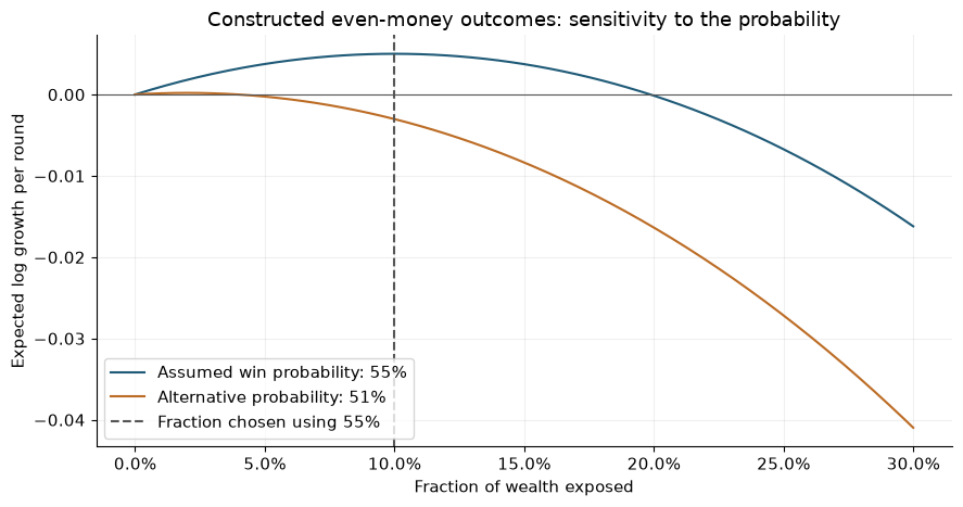
Constructed even-money outcomes. The vertical line marks the 10% fraction selected under the 55% assumption. Neither curve represents observed investment returns.
| Exposure | Fraction of wealth | Log growth at 55% | Log growth at 51% |
|---|---|---|---|
| Full fraction | 10% | 0.005008 | -0.003018 |
| Half fraction | 5% | 0.003753 | -0.000251 |
| Cash | 0% | 0 | 0 |
These are expected logarithmic increments per round, not annualized return forecasts. The optimal fraction at a genuine 51% probability would be only 2%. A seemingly modest four-percentage-point disagreement about probability materially changes the rational size of the position.
The notebook independently compares its numerical optimizer with the binary closed form. The negative values under the weaker edge come directly from the same log-growth formula. The result illustrates sensitivity rather than identifying a recommended investment fraction.
Extending the idea to several assets
For simple-return scenario vectors $r_s$ with probabilities $p_s$, a cash residual and no borrowing, the portfolio problem becomes
\[\max_w\sum_s p_s\log(1+w^\top r_s),\qquad w\geq0,\quad\mathbf1^\top w\leq1.\]Every scenario must satisfy $1+w^\top r_s>0$. The cash residual is part of the decision; forcing risky weights to sum to one changes the feasible set. Gross price relatives are also different from simple returns and cannot be substituted into the wealth expression without changing its meaning.
The notebook includes five original two-asset scenarios with stated probabilities. It checks that probabilities sum to one, all scenario wealth levels remain positive, and risky capital plus cash respects the budget. The result is optimal only for those declared scenarios and constraints. Omitted losses, dependence through time and changing opportunity quality remain outside that finite example.
A second-order approximation to log growth can resemble a mean–variance expression. That relationship does not make clipped and normalized inverse-covariance weights an exact solution to the constrained log-utility problem. The approximation, admissible wealth domain and cash treatment need their own justification.
Turning growth theory into robust allocation research
The central empirical challenge is estimating the distribution well enough to size exposure. A strategy selected from many attractive backtests may have an overstated edge before Kelly sizing even begins. The backtest-selection laboratory demonstrates selection diagnostics on a complete constructed candidate library. It does not provide a missing probability estimate for this example or certify the historical ETF study.
Tail scenarios are equally consequential. Expected-shortfall allocation investigates what happens when an optimizer is asked to manage severe losses that its original scenario set omitted. Volatility targeting offers a different exposure objective, driven by estimated risk rather than an estimated log-growth optimum.
The foundation is Kelly’s 1956 paper. Continue with the research note, worked notebook, or the allocation collection. This chapter supplies checked numerical examples; it does not reuse the legacy notebook’s historical performance claims.