
Hierarchical risk parity organizes an allocation around estimated relationships between assets. It groups similar exposures, orders them through a tree, and divides capital recursively. That structure can make the allocation process easier to inspect than a single optimized weight vector. It also introduces its own choices: distances, linkage, ordering and cluster risk estimates.
The important research question is whether this organization adds value after accounting for the risk it actually takes. In the project’s retrospective ETF study, HRP’s late-segment annualized mean/volatility advantage over its prior-risk-scaled equal-weight control is +0.649, with a paired 95% block interval of [-0.649, +1.954]. The interval includes zero. A neat tree and a small drawdown do not establish incremental allocation value.
From dependence to distance
The maintained construction begins with a return correlation matrix. It converts each correlation into a distance:
\[d_{ij}=\sqrt{\frac{1-\rho_{ij}}{2}}.\]Perfect positive correlation gives distance zero. Lower correlation creates greater separation. Single linkage then groups assets using their pairwise distances, and the tree supplies a leaf order for recursive bisection.
This version still relies on estimated correlations. It is not a replacement for dependence measurement, and the tree does not automatically identify causal economic factors. An industry cluster or bond cluster is an interpretation to investigate, not a label guaranteed by the algorithm.
For each left/right split, estimate cluster variances $v_L$ and $v_R$ using inverse-variance weights within the clusters. Allocate the left cluster the fraction
\[\alpha_L=\frac{v_R}{v_L+v_R},\]and the right cluster $1-\alpha_L$. Repeat until every asset has a weight. The lower-variance cluster receives more capital. This recursive rule differs from explicitly equalizing every asset’s contribution to total portfolio variance.
A tree that can be checked by hand
The worked notebook constructs four assets: two equity exposures with volatilities of 18% and 16%, and two bond exposures at 8% and 6%. Correlations are 0.80 within equities, 0.70 within bonds, and 0.10 across the two groups.
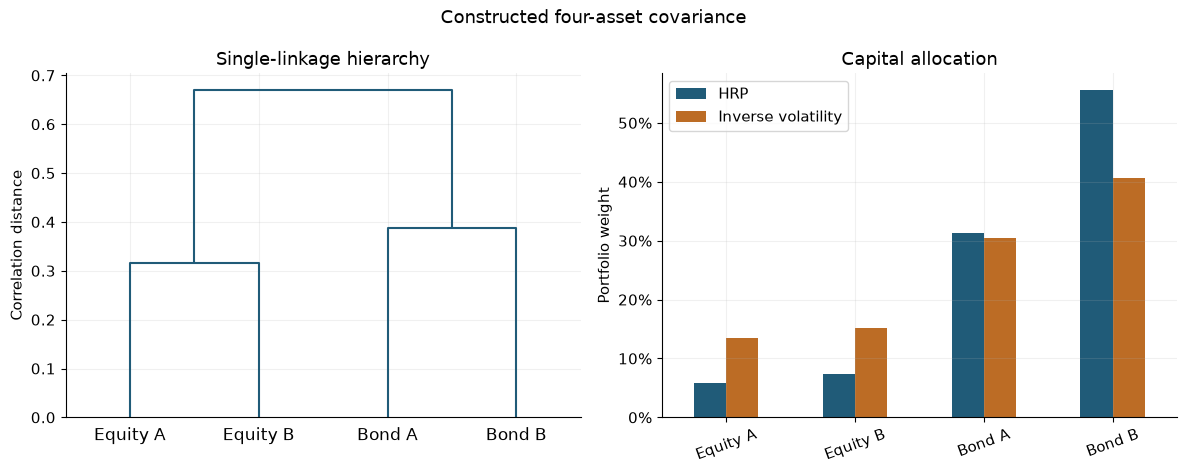
Constructed covariance example. The hierarchy reflects supplied correlations, while the capital allocation also depends on the supplied volatilities.
The tree finds the intended groups, but HRP does not split capital equally between them. It allocates about 13.05% to the equity pair and 86.95% to the bond pair. The least volatile asset, Bond B, receives 55.65% of the portfolio. Structural diversification and capital diversification are different objects.
A two-asset limiting case sharpens the distinction. For diagonal variances 0.04 and 0.01, the split gives weights of 20% and 80%, proportional to inverse variance. Inverse volatility would give one third and two thirds. The notebook checks the former result exactly for its HRP implementation.
It also verifies the clustering input: SciPy receives a condensed vector of pairwise distances. Passing a square distance matrix directly would make the library interpret rows as observations and solve a different clustering problem. The official linkage documentation explains that distinction.
Does lower risk explain the historical result?
The separate ETF case uses US equity, emerging equity, long Treasuries, gold and short Treasuries. Its pinned adjusted-price vintage spans 2 July 2018–17 September 2026. The late evaluation segment is January 2025–17 September 2026; decisions use earlier information, holdings drift, and trades incur costs.
HRP holds substantial short-Treasury exposure. Comparing its risk-adjusted statistic only with fully invested equal weight would mix portfolio construction with a large change in risk. The study therefore scales equal weight using prior covariance estimates, caps risky exposure at 100%, and leaves the remainder in zero-interest cash.
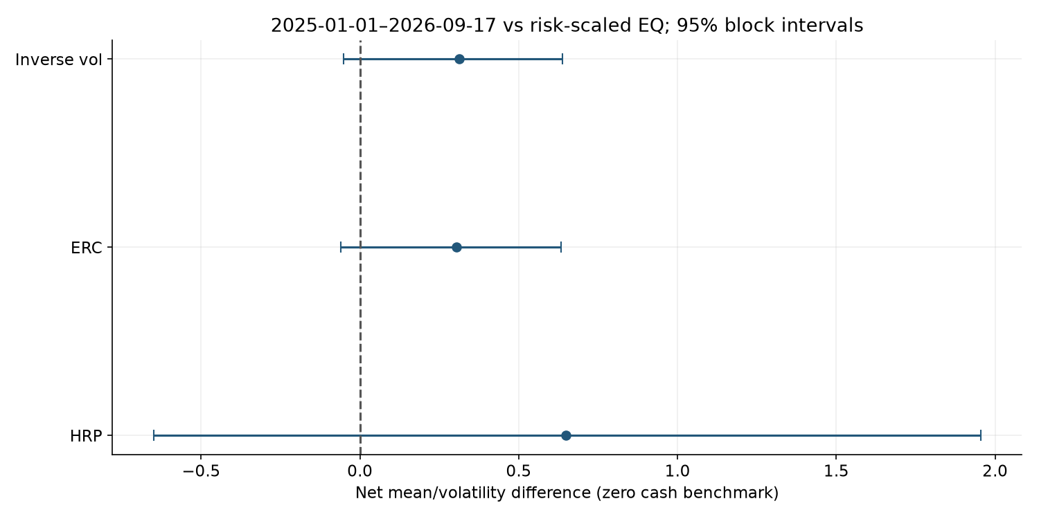
Retrospective late-segment results under the declared execution, cost and zero-cash-interest assumptions. Each row uses its own prior-risk-scaled equal-weight control; HRP is the primary comparison. The intervals resample paired return blocks and do not correct for the complete history of research choices.
The +0.649 estimate is a difference in annualized mean/volatility ratios, not a percentage return and not an observed risk-free-adjusted Sharpe improvement. The uncertainty is wide. Cash also differs economically from a short-bond ETF, and prior risk matching cannot guarantee identical realized risk.
What would make the allocation more convincing?
Avoiding a covariance inverse does not remove estimation risk. A small correlation change can alter the tree; single linkage can join groups through a narrow connection; different tie handling can change ordering. Robustness requires checking these choices and retaining the results when the allocation becomes less attractive.
The estimation-risk laboratory examines sensitivity to perturbed inputs. Factor-risk allocation checks common exposures that asset names can conceal. The historical findings and sensitivity tables retain the uncertain result instead of replacing the primary design with its strongest variant.
Read the original HRP paper for methodological context, then the project note, executed notebook, and allocation research collection.