
This post is about Regime Switching Model for financial market
What is Regime Switching Model
Financial market tend to show different behavior and pattern if market change their state. State is called “regime” in financial market. Easy example of regime switch is quantitative easying after COVID-19 outbreak in 2020, start of quantitative tightening in 2022. If we can determine what the regimes are, we can understand how a portfolio might react to various regime. This can enhance model’s predictability and reduce effort to build all-time effective killer model.
How to build regime switch model
Data-driven approach is letting historical data on assets and/or market risks delineate the regimes. A specific example of this approach is a Gaussian Mixture Model (GMM), which is a type of unsupervised learning method. The GMM uses various Gaussian distributions to model different parts of the data.
Why Gausian Mixture Model for regime switch model
Gausian Mixture Model(GMM) is an especially helpful method for modeling financial assets, as their return distributions can often exhibit skew with a meaningful number of observations in the tails. Clusters derived from Guasian Mixture Model allow us to infer which state market is located at. Better estimation of market regime, more suitable tailored investment strategy and framework can be deployed.
Why Hidden Markov Model for regime switch model
Fitting Market status to cluster(regime) is helpful for understanding current status. However, opportunity in finance domain can be found in prediction of future market. Information about how market regime switch is directly linked to profit of investment strategy.
Data used (index)
I used index data from major index maker. All index are available in ETF(Exchange Traded Fund) form and can be traded easily. Index data can be found from 1992 to 2021.
1
2
3
4
5
 Developed Market : MSCI world
 Emerging Market : MSCI Emerging
 Fixed Income : Bloomberg Barclays World AGG
 Risky Fixed Income : Bloomberg Barclays high yield bond
 Safety Fixed Income : Bloomberg Barclays Short-Term Treasury
Emerging Marekt, Corporate(junk) bond and Safety Treasury effectively distinguished market regime. These assets shows unique movement if market sentiment, regime changes.
Strategy Overview
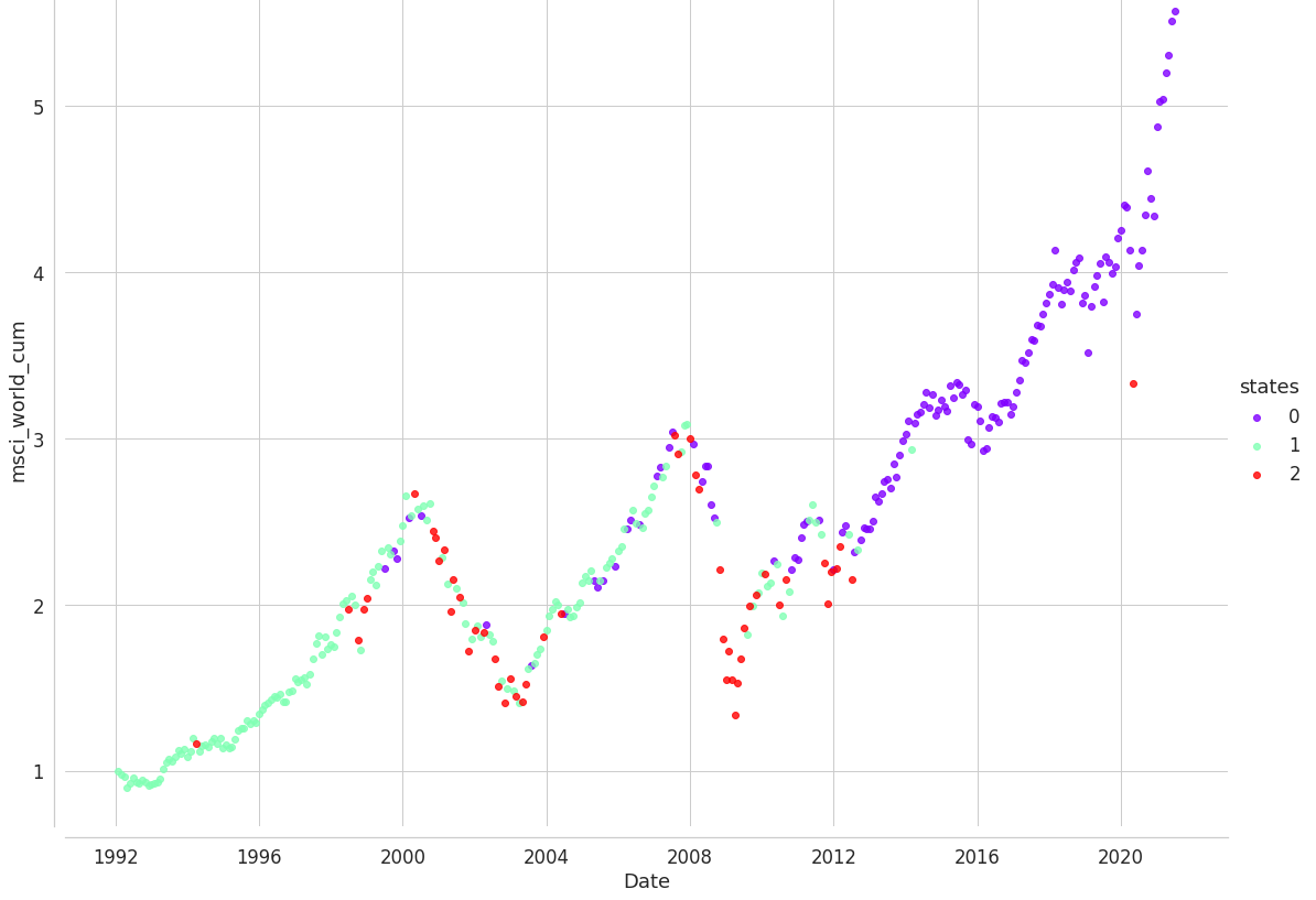
0th hidden state shows bull market regime. 1th hidden state shows sideways stock market regime. 2nd hidden state shows bear market regime. 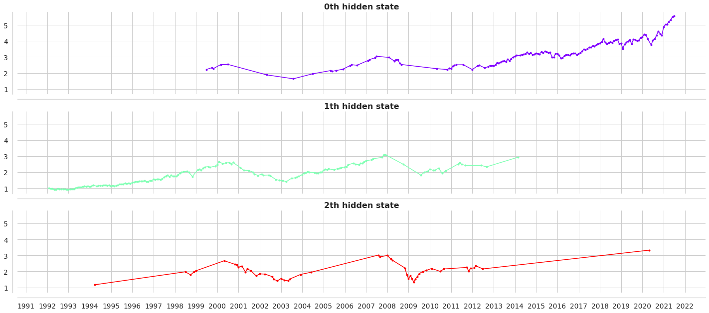
1
2
3
4
5
6
7
8
Asset Class \ State           0th (mean / var)  1th (mean / var)  2nd (mean / var)
--------------------------    ----------------  ----------------  ----------------
mean Emerging Market          7.11433203e-03    0.01311532        -9.92782827e-03
vol  Emerging Market          2.01192349e-03    2.83001901e-03    1.16043600e-02
mean Risky Fixed Income       6.31190614e-03    0.01015012        -1.80401754e-03
vol  Risky Fixed Income       2.71058521e-04    8.79653083e-05    2.41111876e-03
mean Safety Fixed Income      1.24535026e-03    0.00452034        3.97258990e-03
vol  Safety Fixed Income      7.25365976e-06    2.01275656e-05    2.95434611e-05
Full Code
You can see full code in here CODE
Let’s code this idea
Mean variance strategy via python code. We used the networkx package to create Markov chain diagrams, and sklearn’s GaussianMixture to estimate historical regimes
1
2
3
4
5
6
7
8
9
10
11
12
13
14
15
16
17
18
19
20
21
22
23
24
25
26
27
28
29
30
31
32
33
34
35
36
37
38
model = mix.GaussianMixture(n_components=3,
                            covariance_type="full",
                            n_init=100,
                            random_state=8).fit(X)

# Predict the optimal sequence of internal hidden state
hidden_states = model.predict(X)

print("Means and vars of each hidden state")
for i in range(model.n_components):
    print("{0}th hidden state".format(i))
    print("mean = ", model.means_[i])
    print("var = ", np.diag(model.covariances_[i]))
    print()

sns.set(font_scale=1.25)
style_kwds = {'xtick.major.size': 3, 'ytick.major.size': 3,
              'legend.frameon': True}
sns.set_style('whitegrid', style_kwds)

fig, axs = plt.subplots(model.n_components, sharex=True, sharey=True, figsize=(20,9))
colors = cm.rainbow(np.linspace(0, 1, model.n_components))

for i, (ax, color) in enumerate(zip(axs, colors)):
    # Use fancy indexing to plot data in each state.
    mask = hidden_states == i
    ax.plot_date(select.index.values[mask],
                 select[target].values[mask],
                 ".-", c=color)
    ax.set_title("{0}th hidden state".format(i), fontsize=16, fontweight='demi')

    # Format the ticks.
    ax.xaxis.set_major_locator(YearLocator())
    ax.xaxis.set_minor_locator(MonthLocator())
    sns.despine(offset=10)
    # sns.despine(left=True, bottom=True)

plt.tight_layout()
Strategy Evaluation
To be added.