
A high-volatility state estimated from historical returns can help describe market risk. Turning that state into an option price requires another ingredient: the price investors assign to future regime uncertainty. A historical transition matrix alone does not determine this price.
This article revisits Option Pricing with Markov Switching by Cheng-Der Fuh, Kwok Wah Remus Ho, Inchi Hu, and Ren-Her Wang, published in the Journal of Data Science in 2012. The authors develop European-call pricing with finite-state switching and compare discrete-diffusion and Markovian-tree calculations. Their paper remains the source of the option-model discussion; my renovated project contributes a separate historical risk-forecast experiment. It has not calibrated this option model or reproduced the paper’s numerical tables. Original article and PDF.
Two questions, two probability measures
For historical risk, the question is what is likely to happen under the physical probability measure $P$. A switching diffusion might be written
\[\frac{dS_t}{S_t}=\mu_{Z_t}\,dt+\sigma_{Z_t}\,dW_t^P,\]where $Z_t$ is a finite-state Markov chain. Estimation from returns concerns the drift, volatility, and transitions under $P$.
For valuation, the question is how to discount a contingent payoff consistently with a chosen pricing measure $Q$. With constant interest rate $r$, zero dividends, and a specified risk-neutral state process, a state-conditional European call has value
\[C_i(S,T)=e^{-rT}\mathbb E^Q[(S_T-K)^+\mid S_0=S,Z_0=i].\]The stock’s risk-neutral drift becomes $r$, while the transition generator also requires specification under $Q$. Adjusting the drift alone does not identify compensation for regime risk. Fuh and coauthors introduce hypothetical change-of-state securities to identify that compensation within their model. Such securities are an assumption of their pricing construction, not instruments observed or calibrated in my repository. See the paper, Section 2.
This distinction prevents an attractive but unsupported shortcut: fitting an HMM to daily prices and inserting its estimated physical transitions into an option pricer as if they were market-implied transitions.
An occupation-time view of the payoff
The following conditional calculation explains the mechanism without reproducing the paper’s full analytical solution. Assume the state process and Brownian motion are independent under the specified pricing measure, and volatility is constant inside each state. Over remaining maturity $T$, define time spent in state $j$ and accumulated variance:
\[\tau_j=\int_0^T\mathbf{1}\{Z_u=j\}\,du, \qquad V_T=\sum_j\sigma_j^2\tau_j, \qquad \sum_j\tau_j=T.\]Conditional on the state path,
\[\log S_T=\log S+rT-\tfrac12V_T+\sqrt{V_T}\,\varepsilon, \qquad \varepsilon\sim\mathcal N(0,1).\]Its discounted call expectation is therefore
\[c(V_T)=S\Phi(d_1)-Ke^{-rT}\Phi(d_2), \qquad d_1=\frac{\log(S/K)+rT+V_T/2}{\sqrt{V_T}}, \quad d_2=d_1-\sqrt{V_T}.\]Averaging $c(V_T)$ over the risk-neutral state paths yields the call value. The conditional price is nonlinear in accumulated variance, so substituting only its mean generally loses information. This is the economic reason the entire occupation-time distribution matters. The expression also keeps the initial stock price in exactly one place: multiplying by an additional $S$ after already including $\log S$ inside a lognormal mean would double-count it.
The occupation-time law includes point masses for paths that never switch. A numerical integral using only a smooth density can omit those paths and misprice short maturities. Equal state volatilities give $V_T=\sigma^2T$ for every path and recover the ordinary Black–Scholes value; zero switching reduces the calculation to the initial state’s value. These are natural mathematical checks before attempting calibration.
State uncertainty remains a modeling choice
The paper’s observability argument uses ideal continuous observation and distinct local variances. Daily closes provide much less information. In my empirical project, the state remains a probability distribution updated after each close; it is not assigned an economic label such as expansion or recession.
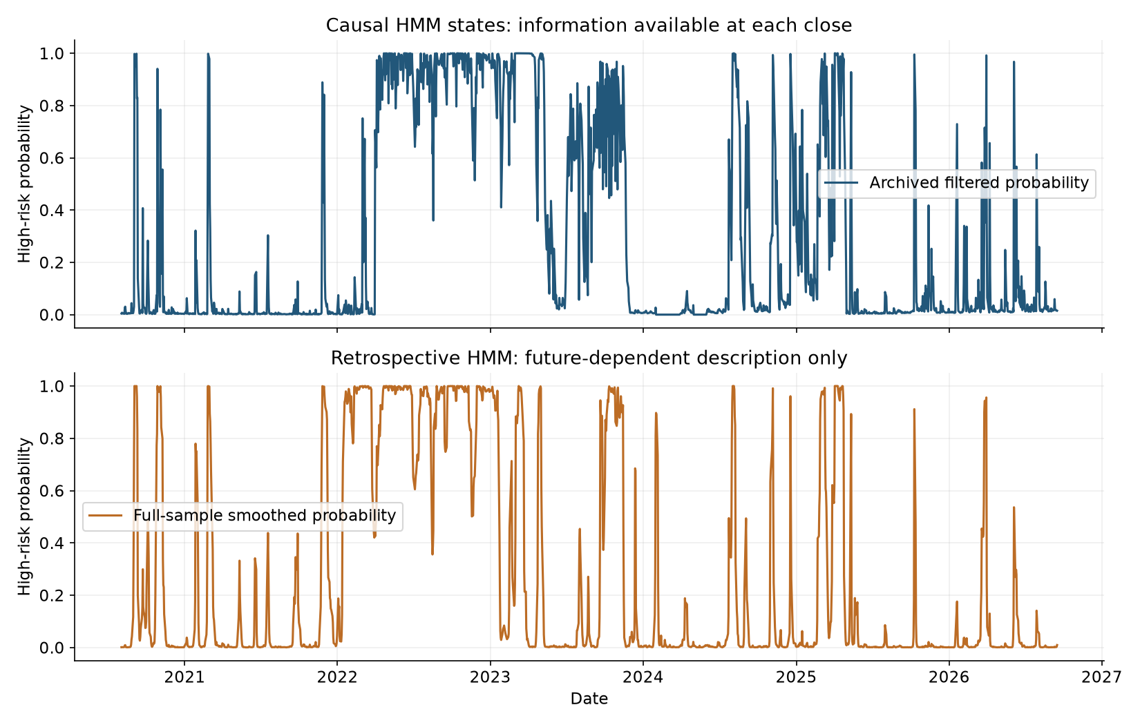
This original figure comes from the historical equity-risk study. It illustrates information dependence in state inference, not an option-price calibration or a risk-neutral probability estimate.
The two panels differ on 15.28% of hard labels after thresholding at 0.5. The full-sample calculation changes both fitted parameters and conditioning information. Using that retrospective state history as a live pricing input would require information unavailable at the original valuation time.
Likewise, a fitted discrete-time transition matrix is not automatically a continuous-time pricing generator. A valid generator must have nonnegative off-diagonal entries and zero row sums; a proposed conversion and its time units require explicit checks. A combined model needs consistent state definitions and observation assumptions while keeping its probability measures distinct.
What the renovated project establishes
The completed experiment uses S&P 500 and long-maturity Treasury fund returns, with training-only scaling, monthly refits, and archived forward filters. On 428 next-session equity risk forecasts from January 2025 through 17 September 2026, HMM-minus-EWMA mean loss is +0.2539, with a 95% block interval of [−0.1024, +0.8795]. It does not establish an improvement over the simple volatility baseline. The data are revised historical snapshots; the evaluation is retrospective. Methods and actual results.
That finding neither validates nor rejects the option-pricing model: historical forecast loss and risk-neutral pricing error are different endpoints. A useful next option experiment would freeze dated option quotes and conventions, compare prices across strikes and maturities, check put–call parity and numerical convergence, then evaluate hedges on later observations with transaction costs. Parameter stability and bid–ask spreads would determine whether a lower calibration error matters economically.
Those option experiments remain unrun. Readers can inspect the completed regime notebook and research protocol, then return to the original paper for the option-specific derivation. Keeping that boundary explicit makes both the theory and the empirical evidence more useful.