
A strong leading asset can coexist with growing weakness elsewhere in a portfolio’s opportunity set. Vigilant Asset Allocation makes that breadth part of the decision. Relative strength selects a holding; the number of weak assets determines how much capital remains in risky holdings.
The controlled example in this chapter leaves the strongest asset unchanged while weakening a different asset. Under the chosen breadth threshold, that single change switches the entire allocation from the leading risky asset into the strongest defensive asset. The mechanism is easy to inspect, but it also exposes the central research risk: the monitored universe can determine exposure even through assets that would never be selected.
Measure strength with a price-based score
The notebook uses returns over one, three, six and twelve months:
\[R_{h,t}=\frac{P_t}{P_{t-h}}-1.\]It combines them in the unscaled momentum score
\[M_t=12R_{1,t}+4R_{3,t}+2R_{6,t}+R_{12,t}.\]The heavier emphasis on recent performance makes a reversal affect the score quickly. The result is a composite ranking measure, not a predicted annual return. A common positive rescaling leaves its rankings and zero threshold unchanged.
Prices are essential to this definition. Dividing one daily return by another does not calculate trailing momentum and can behave badly near a zero return. The executed notebook checks the four-horizon score against an independently calculated constant-growth path and rejects missing or nonpositive price inputs.
Count weakness before assigning capital
Let $b_t$ count assets with non-positive momentum inside the risky universe. For a declared breadth threshold $B$, the fractional illustration assigns
\[d_t=\min\left(1,\frac{b_t}{B}\right)\]to the defensive sleeve. The strongest risky asset receives $1-d_t$, and the strongest defensive asset receives $d_t$.
The primary example uses four fictional risky exposures, two defensive exposures, one risky holding and $B=1$. Every risky score must be positive to remain fully invested in the leading risky asset. A score of exactly zero counts as weak. A separate $B=2$ illustration permits half the portfolio to remain risky when exactly one score is weak.
This is a transparent teaching specification inspired by the original VAA paper. The fractional $B=2$ case does not reproduce all portfolio-slot rounding conventions in the published variants, and neither case claims their historical performance.
Keep the leader fixed and change participation
The notebook creates three twelve-month scenarios. The first has broadly positive momentum. The second changes only the final return of the emerging-equity exposure. The third introduces broader weakness.
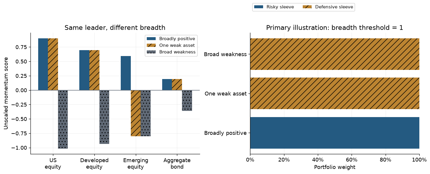
Constructed price paths and signal snapshots. The right panel uses the primary breadth threshold of one. No investment return series is inferred from these snapshots.
| Scenario | Weak risky assets | Defense with $B=1$ | Defense with $B=2$ |
|---|---|---|---|
| Broadly positive | 0 | 0% | 0% |
| One weak asset | 1 | 100% | 50% |
| Broad weakness | 4 | 100% | 100% |
In the first two scenarios, the US-equity score remains about 0.9006 and leads the risky assets. Emerging equity changes from about +0.5920 to -0.8019. The leader remains attractive under its own score, but the deterioration elsewhere changes the portfolio’s exposure budget. The defensive ranking then determines what replaces the risky holding; the example selects its constructed Treasury exposure.
Budget checks confirm that weights remain nonnegative and sum to one. The notebook also checks the zero threshold, future-price invariance and the sequence from information at month 12 to execution at month 13 and the first earned return ending at month 14. These checks support the mechanism’s integrity, not a prediction of successful market timing.
The economic cost of responding early
A sensitive breadth threshold can trigger defense before the current leader weakens. It can also cause repeated exits, late re-entry and missed recoveries. Changing the asset universe changes the count: adding another correlated exposure may create an additional vote without much independent information.
The defensive asset has its own risks. A Treasury holding responds to interest rates, and a bond fund is not equivalent to cash. Assessing a detector requires examining both the losses it avoids and the gains it misses, alongside turnover and the behavior of the replacement asset.
A robust empirical design would fix the universe, score, breadth threshold, holdings count and execution rule before evaluation. It would retain unsuccessful parameter variants and distinguish a deliberately defined later sample from a history already inspected. The repository’s separate ETF case uses its own defensive-momentum adaptation; its results should not be reassigned to this VAA illustration.
Continue to defensive allocation and canary signals to separate the monitored universe from the holdings universe. Volatility targeting changes exposure using estimated risk instead of breadth. The VAA research note, worked notebook, and allocation research collection provide the connected examples.