
This post is about risk parity asset allocation strategy.
What is Risk Parity strategy
Risk parity(Equally weighted risk contribution portfolio) is commonly used in asset allocation strategy. Goal of this strategy is to allocate same amount of risk to each asset classes.
Consider portfolio of N assets. $(x_1,x_2,x_3,x_4, … ,x_N)$, where weight of assets $x_i$ is $w_i$, and standard deviation of the asset $x_i$ is $std_i$.
Goal of this portfolio is not to find portfolio X which satisfy $\sigma_1 = \sigma_2 = … = \sigma_N$ ). Covariance of each asset classes in portfolio should be considered.
Let us note covariance matrix of the assets $X = (x_1, x_2, …, x_N)$ by $\sum$ and risk contribution of each asset as $\sigma_i$. The volatility of the portfolio is defined as $\sigma(x) = \sum = \sqrt{w’ \sum w}$ which is homogeneous of degree 1. Thus following Euler’s theorm for homogeneous function.
$ \sigma_p(w) =\sum = \sqrt{w’ \sum w} = \sum_{1=0}^{N} \sigma_i (w) $
$ c(w) = \frac{w_i’ \sigma w_i}{\sqrt{w’\sum w}} = \textsf{marginal risk contribution of asset i} $
$ w_i = \frac{\sigma(w)^2}{(\sum w_i) \cdot N} $
To sum up, we need to solve below formula to return realistic portfolio which contains constraints.
$ \underset{w}{\arg \min} \sum_{i=1}^N [\frac{\sqrt{w^T \Sigma w}}{N} - w_i \cdot c(w)_i]^2 $
How Risk Parity strategy works?
Let’s check how this strategy works. First of all, I will compare how risk parity strategy will differ from traditional 60:40 strategy. Traditional 60:40 strategy derived from mean-variance optimization. While mean-variance optimization aims to maximize shapre ratio, Risk-parity optimization aims to build equal risk contribution. See illustration below 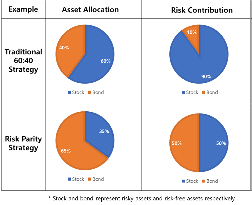
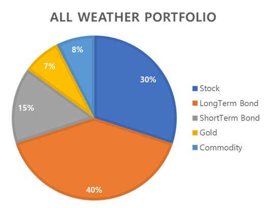
Similar to risk parity strategy, all weather strategy targets all time(regime) available strategy. These strategies’ goals are similar since they both target all time, all asset classes working strategy. In addition, both strategy contains lots of gold in their portfolio. The gold in portfolio shows different but stable investment performance from stock and bond.
Data used and Benchmark for this strategy
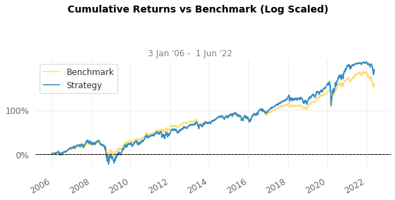
I used index data from major index maker. Date from Jan 2006 to July 2022. All index are available in ETF(Exchange Traded Fund) form and can be traded easily. And benchmark for this strategy is 1/N portfolio.
1
2
3
4
5
6
7
8
9
10
 US Equity Market: SPDR S&P 500 ETF Trust(SPY)
 Developed Market: iShares MSCI EAFE ETF(EAF)
 Emerging Market: iShares MSCI Emerging Markets ETF(EEM)
 Short Term Bond: iShares 1-3 Year Treasury Bond ETF(SHY)
 Long Term Bond: iShares 7-10 Year Treasury Bond ETF(IEF)
 Ultra Long Term Bond: Shares 20+ Year Treasury Bond ETF (TLT)
 IG Corporate Bond: iShares iBoxx Investment Grade Corporate Bond ETF(LQD)
 TIPS Bond: iShares TIPS Bond ETF(TIP)
 Real Estate: Vanguard Real Estate Index Fund(VNQ)
 Gold: SPDR Gold Shares(GLD)
Backtesting Detail
Monthly rebalancing is assumed. To calculate portfolio, I used 12 month past data to derive covariance matrix(lookup period = 12 month). Portfolio weight has sup/inf constraints which is (30%, 5%)
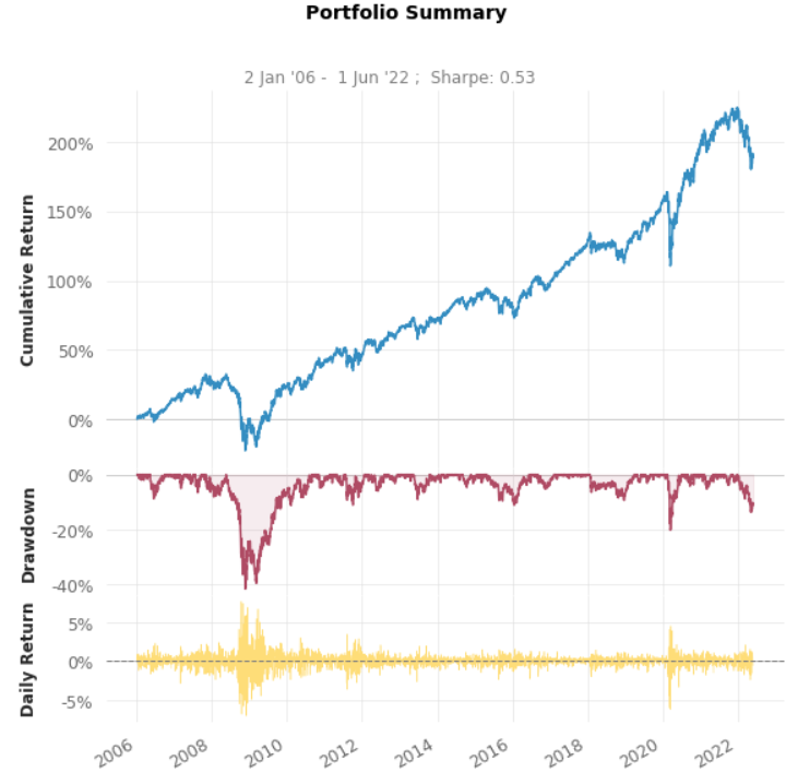
Strategy Overview
1
2
3
4
5
6
7
8
                           Strategy    Benchmark
-------------------------  ----------  -----------
Start Period               2006-01-03  2006-01-03
End Period                 2022-06-01  2022-06-01

Cumulative Return          188.74%     157.28%
CAGR﹪                     6.67%       5.92%
Sharpe                     0.53        0.66
Full Code
You can see full code in here CODE
Let’s code this idea
Risk parity strategy via python code.
1
2
3
4
5
6
7
8
9
10
11
12
13
14
15
16
17
18
19
20
21
22
23
24
25
26
27
28
29
30
31
32
33
34
35
36
37
38
39
40
41
42
43
44
45
46
47
48
49
50
51
52
53
54
def RiskParity(covariance_matrix):

  # Calculate risk parity
  # :param covariance_matrix: covariance matrix of assets in universe
  # :return: [list] weight of risk parity investment strategy

  x0 = np.repeat(1/covariance_matrix.shape[1], covariance_matrix.shape[1])
  constraints = ({'type': 'eq', 'fun': SumConstraint},
                {'type': 'ineq', 'fun': LongOnly})
  options = {'ftol': 1e-20, 'maxiter': 2000}

  result = minimize(fun = RiskParityObjective,
                    args = (covariance_matrix),
                    x0 = x0,
                    method = 'SLSQP',
                    constraints = constraints,
                    options = options)
  return result.x

def RiskParityObjective(x, covariance_matrix) :
  # x means weight of portfolio
  variance = (x.T) @ (covariance_matrix) @ (x)
  sigma = np.sqrt(variance)
  mrc = 1/sigma * (covariance_matrix @ x)
  risk_contribution = x * mrc
  a = np.reshape(risk_contribution.to_numpy(), (len(risk_contribution), 1))

  # set marginal risk level of asset classes equal
  risk_diffs = a - a.T
  # np.ravel: convert n-dim to 1-dim
  sum_risk_diffs_squared = np.sum(np.square(np.ravel(risk_diffs)))
  return (sum_risk_diffs_squared)

# constraint 1 : sum of weight should be less than equal to 1
def SumConstraint(weight):
  return (weight.sum()-1.0)

# constraint 2 : long only portfolio should be consists of postive weight vectors
def LongOnly(weight):
  return(weight)

def RiskContribution(weight, covariance_matrix) :
  # to check whether given portfolio is equally distributed
  # :param weight: asset allocation weight of portfolio
  # :param covariance_matrix:
  # :return: risk contribution of each asset
  weight = np.array(weight)
  variance = np.dot(np.dot(weight.T, covariance_matrix) ,weight)
  sigma = np.sqrt(variance)
  mrc = 1/sigma * np.dot(covariance_matrix, weight)

  risk_contribution = weight * mrc
  risk_contribution = risk_contribution / risk_contribution.sum()
  return risk_contribution
Full Result
1
2
3
4
5
6
7
8
9
10
11
12
13
14
15
16
17
18
19
20
21
22
23
24
25
26
27
28
29
30
31
32
33
34
35
36
37
38
39
40
41
42
43
44
45
46
47
48
49
50
51
52
53
54
55
56
57
58
59
60
61
62
63
                           Strategy    Benchmark
-------------------------  ----------  -----------
Start Period               2006-01-03  2006-01-03
End Period                 2022-06-01  2022-06-01
Risk-Free Rate             0.0%        0.0%
Time in Market             100.0%      100.0%

Cumulative Return          188.74%     157.28%
CAGR﹪                     6.67%       5.92%

Sharpe                     0.53        0.66
Prob. Sharpe Ratio         98.33%      99.62%
Smart Sharpe               0.45        0.57
Sortino                    0.75        0.95
Smart Sortino              0.64        0.81
Sortino/√2                 0.53        0.67
Smart Sortino/√2           0.46        0.57
Omega                      1.11        1.11

Max Drawdown               -41.67%     -28.05%
Longest DD Days            1037        540
Volatility (ann.)          14.22%      9.36%
R^2                        0.91        0.91
Information Ratio          0.01        0.01
Calmar                     0.16        0.21
Skew                       0.06        -0.07
Kurtosis                   13.33       10.42

Expected Daily %           0.03%       0.02%
Expected Monthly %         0.54%       0.48%
Expected Yearly %          6.44%       5.72%
Kelly Criterion            4.33%       5.96%
Risk of Ruin               0.0%        0.0%
Daily Value-at-Risk        -1.44%      -0.95%
Expected Shortfall (cVaR)  -1.44%      -0.95%

Max Consecutive Wins       12          15
Max Consecutive Losses     10          9
Gain/Pain Ratio            0.11        0.13
Gain/Pain (1M)             0.74        0.83

Payoff Ratio               0.9         0.91
Profit Factor              1.11        1.13
Common Sense Ratio         1.05        1.05
CPC Index                  0.55        0.57
Tail Ratio                 0.94        0.93
Outlier Win Ratio          4.05        5.77
Outlier Loss Ratio         3.73        5.33

MTD                        -0.55%      -0.46%
3M                         -6.32%      -6.63%
6M                         -8.66%      -8.68%
YTD                        -11.02%     -10.6%
1Y                         -6.9%       -7.44%
3Y (ann.)                  6.49%       4.36%
5Y (ann.)                  6.48%       4.9%
10Y (ann.)                 6.8%        4.75%
All-time (ann.)            6.67%       5.92%

Beta                       1.45        -
Alpha                      -0.02       -
Correlation                95.55%      -
Treynor Ratio              130.0%      -
Weight flow of portfolio over investment horizon 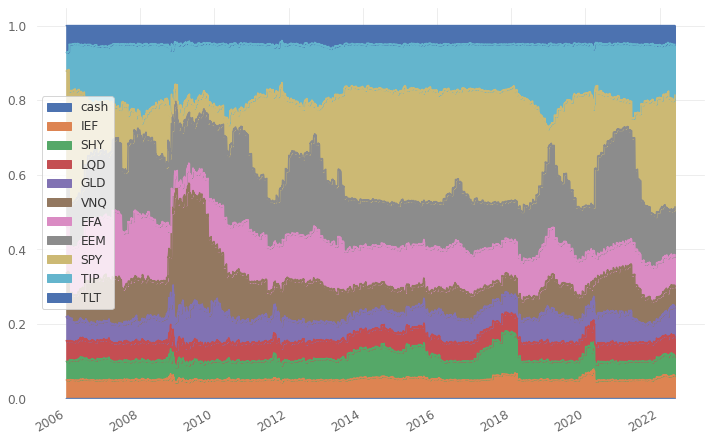
Distribution of the strategy and the benchmark 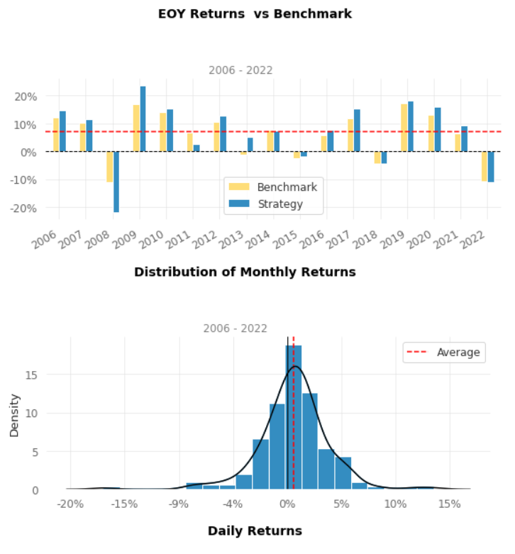
Monthly analysis of historical performance 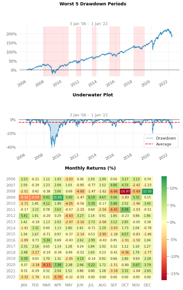
Strategy Evaluation
Evaluating investment strategy can be differ by investors and metrics. For high frequency trader, absoulte return is sole metric to evaluate the strategy. For long term investors, however other than absolute return should be considered. Such as risk, turnover, diversification ,,, and so on. Thus, less profitability doesn’t mean that the strategy is not good.
Interesting fact is that, it showed greater returns but showed less attractive risk adjusted return compare to 1/N portfolio. Eventhough I set minimum and maximum weight allocation for each asset classes, it showed quite fluctuation at specific times such as COVID-19.
One thing more interesting is that, risk parity strategy acted little bit insensitive (later) to major regime shift. Since I used past 12 month data to calculate target portfolio, the strategy need time. This parameter so called lookup period can affect greatly to result of portfolio. I personally recommend change this parameter to 1M, 3M, 6M, 12M to check whether this strategy is robust or not.
It is hard to predict the future performance of asset classes. Risk parity approach overcomes this shortcoming by building portfolios using only assets’ risk characteristics and correlation matrix. This idea give great relief to investors that they are suitably allocalte their wealth to major asset classes no matter how the asset classes perform.