This post is about application of Relative(Cross-Sectional) Momentum in Defensive Asset Allocation to financial investors.
What is Momentum
Momentum is defined as product of the mass of a particle and its velocity. Momentum is a vector quantity; i.e., it has both magnitude and direction. From Newton’s second law it follows that, if a constant force acts on a particle for a given time, the product of force and the time interval (the impulse) is equal to the change in the momentum. Conversely, the momentum of a particle is a measure of the time required for a constant force to bring it to rest. Definition of Momentum
In finance domain, momentum means price movement trend. Stock price literally do “work” by forces (probably by market participants). If forces act on stock price, it will move up or down. If stock price move(both with magnitude and quantity) by forces. So, Mid-term momentum means stock price movement trend for mid-term period and Long-term means stock price movement trend for long-term period. Direction can be either postive to negative.
Define Momentum Score DAA
Rule is simple, DAA momentum score is time weighted momentum score. More weight to recent momentum and less weight to past.
Interesting point is that, there is canaria asset which detect anormaly of market in advance.
Stock Price At Time(t) = $ Y_t $
12 Month Momentum= $\frac{Y_t}{Y_(t-12)} - 1$
6 Month Momentum= $\frac{Y_t}{Y_(t-6)} - 1$
3 Month Momentum= $\frac{Y_t}{Y_(t-3)} - 1$
1 Month Momentum= $\frac{Y_t}{Y_(t-1)} - 1$
$ M_i $ = Defensive Asset Allocation Momentum Score
$ M_i $ = 12x(1 Month Momentum) + 4x(3 Month Momentum) + 2x(6 Month Momentum) + 1x(12 Month Momentum)
If Canaria asset shows negative momentum score, the strategy escape to safe heaven. Others build 1/N portfolio with risk assets.
Who invented this idea?
Prof. Wouter J. Keller invented this strategy at 2018. You can see original paper in SSRN. this is revised version of VAA strategy. You can download orignal paper in below url.
Paper
1
2
3
4
5
6
7
8
9
10
11
12
13
14
15
16
17
18
19
# Ofensive Assets
IVV : iShares Core S&P 500 ETF                             2000-05-15
EFA : iShares MSCI EAFE ETF                                2001-08-02
EEM : iShares MSCI Emerging Markets ETF                    2003-04-07
TLT : iShares 20+ Year Treasury Bond ETF                   2002-07-22
RWR : SPDR® Dow Jones® REIT ETF                            2001-04-23
LQD : iShares iBoxx $ Investment Grade Corporate Bond ETF  2002-07-22

# Defensive Assets
SHY : iShares 1-3 Year Treasury Bond ETF                    2002-07-22
IEF : iShares 7-10 Year Treasury Bond ETF                   2002-07-22

# Canaria Assets
EEM : iShares MSCI Emerging Markets ETF                     2003-04-07
IEF : iShares 7-10 Year Treasury Bond ETF                   2002-07-22

# Bechmark for this strategy is 60/40 portfolio
IVV : iShares Core S&P 500 ETF                              2000-05-15
AGG : iShares Core U.S. Aggregate Bond ETF                  2003-09-22
Strategy Overview _ DAA
1
2
3
4
5
6
7
8
9
10
11
Strategy Benchmark
------------------------- ---------- -----------
Start Period 2006-01-03 2006-01-03
End Period 2022-09-30 2022-09-30
Cumulative Return 132.74% 191.11%
CAGR﹪ 5.17% 6.59%
Sharpe 0.61 0.6
Volatility (ann.) 8.93% 11.74%
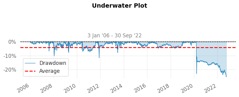
Max Drawdown -25.35% -35.47%
Full Code
You can see full code in here CODE
Let’s code this idea
Vigiliant Asset Allocation with relative Momentum Criterion in multiple asset classes via python code.
1
2
3
4
5
6
7
8
9
10
11
12
13
14
15
16
17
18
19
20
21
22
23
24
25
26
27
28
29
30
31
32
33
34
35
36
37
38
39
40
41
42
43
44
45
46
47
48
49
50
51
52
53
54
55
56
57
58
59
60
61
62
63
64
65
66
67
68
69
70
71
72
73
74
75
76
77
78
79
80
81
82
83
84
85
86
87
88
89
90
91
92
93
94
95
96
97
98
99
100
101
102
103
104
105
106
107
108
109
110
111
112
def get_momentum(self, yld_df):
    """
    calculate momentum of sectors. use 12 month, 6 month, 3 month momentum to bit market
    input
    yiled_df : dataframe with weekly yield of asset classes

    returns : momentum in pandas dataframe format. momentum of each asset classes for give date
    """
    momentum = pd.DataFrame(columns=yld_df.columns, index=yld_df.index)

    windows = 250
    for ticker in yld_df.columns:
        i = 0
        for date in yld_df.index:
            # 250 days before = 1 year  before
            if i > windows :
                # first 12 month data (52 data points) cannot be used since 12 month lagged returns is required
                momentum.loc[date, ticker] = yld_df[ticker].iloc[i] / yld_df[ticker].iloc[i - windows] - 1

                current = yld_df[ticker].iloc[i]
                before_1m = yld_df[ticker].iloc[i-20]
                before_3m = yld_df[ticker].iloc[i-60]
                before_6m = yld_df[ticker].iloc[i-120]
                before_12m = yld_df[ticker].iloc[i-250]

                momentum.loc[date, ticker] = 12*(current/before_1m - 1) + 4*(current/before_3m - 1) \
                                            + 2*(current/before_6m - 1) + 1*(current/before_12m - 1)

            else:
                momentum.loc[date, ticker] = 0
            i = i + 1

    momentum = momentum.replace([np.inf], 1000)
    momentum = momentum.replace([-np.inf], -1000)
    momentum = momentum.replace([np.nan], 0)
    return momentum

def select_sector(self, yld_df):
    """
    select top scored two offensive sectors if condition satisfied(canaria not dead).
    If failed to save canaria, escape to Defensive strategy.

    Criteria: if any of canaria asset classes show negative momentum score, escape to canaria assets.

    returns: selected_tickers in list format. list with top 5 momentum in given period`
    """
    momentum_df = self.get_momentum(yld_df)

    selected_momentum = pd.DataFrame(
        columns=['momentum_1','momentum_2'],
        index=momentum_df.index
    )
    selected_ticker = pd.DataFrame(
        columns=['momentum_1','momentum_2'],
        index=momentum_df.index
    )

    selectable_asset = [
    "IVV",  # iShares Core S&P 500 ETF                              2000-05-15
    "EFA",  # iShares MSCI EAFE ETF                                 2001-08-02
    "EEM",  # iShares MSCI Emerging Markets ETF                     2003-04-07
    "TLT",  # iShares 20+ Year Treasury Bond ETF                    2002-07-22
    "RWR",  # SPDR® Dow Jones® REIT ETF                             2001-04-23
    "LQD",  # iShares iBoxx $ Investment Grade Corporate Bond ETF   2002-07-22
    ]
    # print("emerging market signal : Total ",momentum_df.count()[0])
    # print("postive signal : ", momentum_df[momentum_df['EEM'] >= 0]['EEM'].count())
    # print("negative signal : ", momentum_df[momentum_df['EEM'] < 0]['EEM'].count())


    # print("bond market signal : Total ",momentum_df.count()[0])
    # print("postive signal : ", momentum_df[momentum_df['TLT'] >= 0]['TLT'].count())
    # print("negative signal : ", momentum_df[momentum_df['TLT'] < 0]['TLT'].count())


    for date in momentum_df.index:
        emerging_momentum = momentum_df.loc[date,'EEM']
        bond_momentum = momentum_df.loc[date,'IEF']

        short_treasury_momentum = momentum_df.loc[date,'SHY']
        mid_treasury_momentum = momentum_df.loc[date,'IEF']

        sorted_momentum = momentum_df[selectable_asset].loc[date].sort_values(ascending=False)

        if emerging_momentum >= 0 and bond_momentum >= 0:
            selected_momentum.loc[date,'momentum_1'] = sorted_momentum[0]
            selected_ticker.loc[date,'momentum_1'] = sorted_momentum.index[0]

            selected_momentum.loc[date,'momentum_2'] = sorted_momentum[1]
            selected_ticker.loc[date,'momentum_2'] = sorted_momentum.index[1]

        else:
            selected_momentum.loc[date,'momentum_1'] = short_treasury_momentum
            selected_ticker.loc[date,'momentum_1'] = 'SHY'

            selected_momentum.loc[date,'momentum_2'] = mid_treasury_momentum
            selected_ticker.loc[date,'momentum_2'] = 'IEF'

    return selected_ticker

def daa_momentum(self, yld_df):
    """
    returns : market portfolio in pandas dataframe format.
    """
    mom_ticker_df = self.select_sector(yld_df)
    mp_table = pd.DataFrame(columns=yld_df.columns, index=yld_df.index)
    for date in mom_ticker_df.index:
        selected = mom_ticker_df.loc[date].tolist()
        for sel in selected:
            mp_table.loc[date, sel] = 1/2
    mp_table = mp_table.fillna(0)
    return mp_table
Result of VAA strategy with graphics 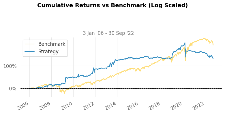
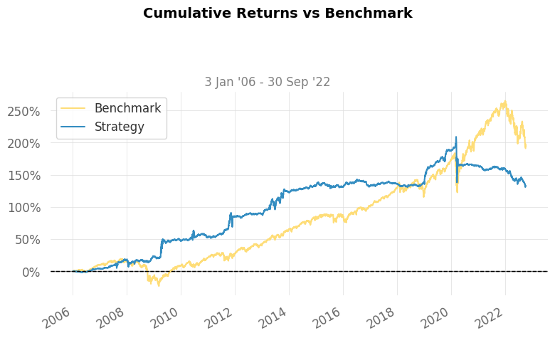
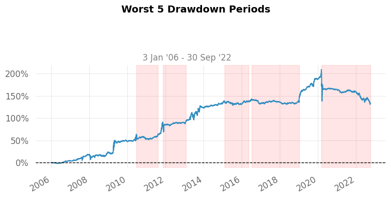
The strategy avoided the most severe losses but missed some of upside movements.
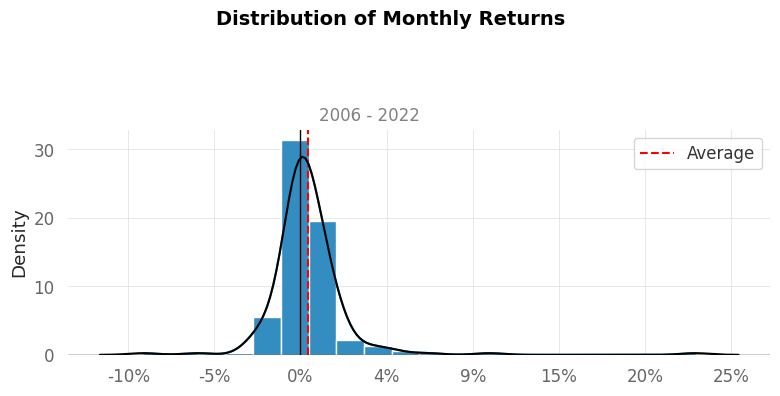
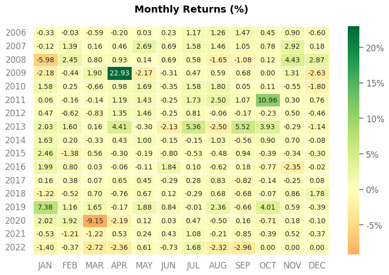
The strategy succesfully eliminated left tail thus distribution shows skewness.
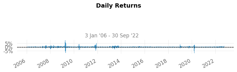
Daily changes of strategy.
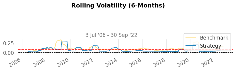
Information for risk averse investors.
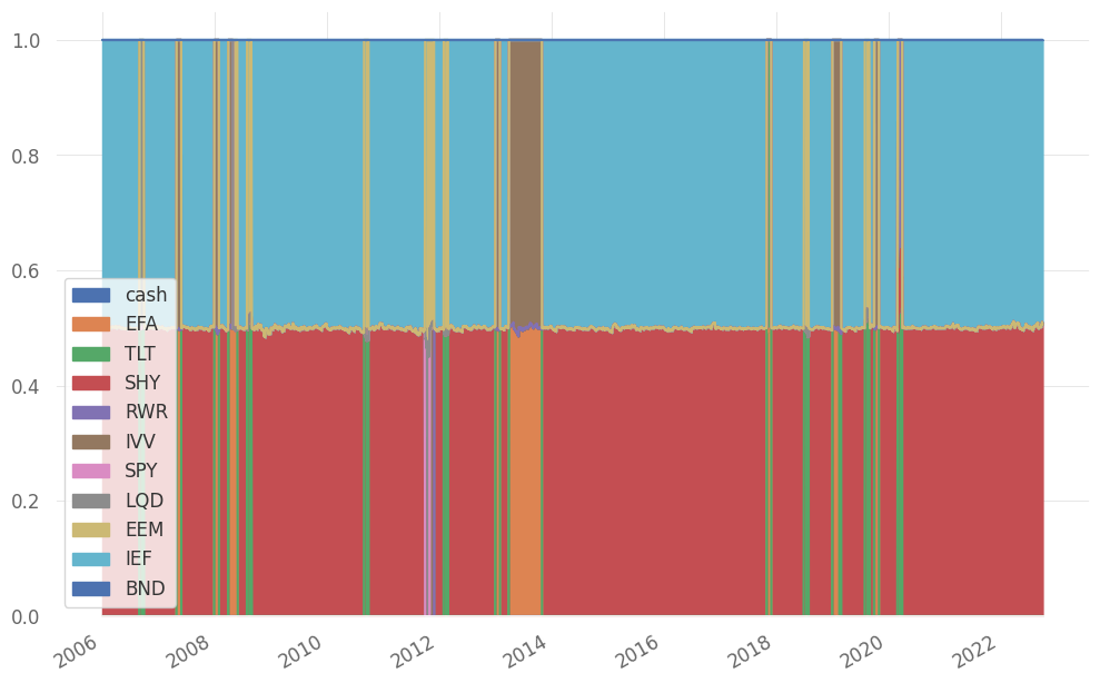
How this strategy allocated portfolio weight for last 15 years?
Full Result
1
2
3
4
5
6
7
8
9
10
11
12
13
14
15
16
17
18
19
20
21
22
23
24
25
26
27
28
29
30
31
32
33
34
35
36
37
38
39
40
41
42
43
44
45
46
47
48
49
50
51
52
53
54
55
56
57
58
59
60
61
62
63
64
65
66
67
68
69
70
71
72
73
74
75
76
77
78
79
80
81
Start Period 2006-01-03 2006-01-03
End Period 2022-09-30 2022-09-30
Risk-Free Rate 0.0% 0.0%
Time in Market 100.0% 100.0%
Cumulative Return 132.74% 191.11%
CAGR﹪ 5.17% 6.59%
Sharpe 0.61 0.6
Prob. Sharpe Ratio 99.31% 99.28%
Smart Sharpe 0.59 0.58
Sortino 0.88 0.84
Smart Sortino 0.86 0.81
Sortino/√2 0.63 0.59
Smart Sortino/√2 0.61 0.58
Omega 1.18 1.18
Max Drawdown -25.35% -35.47%
Longest DD Days 935 1121
Volatility (ann.) 8.93% 11.74%
R^2 0.04 0.04
Information Ratio -0.01 -0.01
Calmar 0.2 0.19
Skew -0.05 -0.29
Kurtosis 63.9 13.1
Expected Daily % 0.02% 0.03%
Expected Monthly % 0.42% 0.53%
Expected Yearly % 5.09% 6.49%
Kelly Criterion -1.43% 6.17%
Risk of Ruin 0.0% 0.0%
Daily Value-at-Risk -0.9% -1.19%
Expected Shortfall (cVaR) -0.9% -1.19%
Max Consecutive Wins 9 13
Max Consecutive Losses 9 8
Gain/Pain Ratio 0.18 0.13
Gain/Pain (1M) 1.19 0.75
Payoff Ratio 0.85 0.92
Profit Factor 1.18 1.13
Common Sense Ratio 1.35 1.03
CPC Index 0.53 0.57
Tail Ratio 1.15 0.92
Outlier Win Ratio 6.47 3.85
Outlier Loss Ratio 7.24 3.87
MTD -2.96% -7.19%
3M -3.16% -5.05%
6M -5.71% -16.9%
YTD -10.19% -20.0%
1Y -10.34% -15.39%
3Y (ann.) -6.85% 3.68%
5Y (ann.) -0.32% 5.56%
10Y (ann.) 2.07% 7.49%
All-time (ann.) 5.17% 6.59%
Best Day 8.93% 7.5%
Worst Day -8.24% -7.23%
Best Month 22.93% 8.64%
Worst Month -9.15% -10.89%
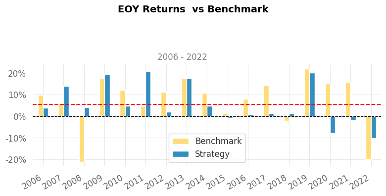
Best Year 20.7% 21.94%
Worst Year -10.19% -21.03%
Avg. Drawdown -1.37% -1.08%
Avg. Drawdown Days 39 18
Recovery Factor 5.24 5.39
Ulcer Index 0.07 0.07
Serenity Index 0.78 1.44
Avg. Up Month 1.51% 2.26%
Avg. Down Month -1.32% -2.82%
Win Days % 53.32% 55.07%
Win Month % 57.21% 67.16%
Win Quarter % 62.69% 71.64%
Win Year % 76.47% 82.35%
Beta 0.16 -
Alpha 0.04 -
Correlation 21.2% -
Treynor Ratio 823.1% -
Strategy Evaluation
As shown above, Defensive Asset Allocation strategy shows pretty unsatisfying returns from COVID-19. Also, unlike previous market correction, this strategy couldn’t avoided COVID-19. This makes me suspicious about this strategy. Furthermore, Canaria asset classes alerts so frequently that this strategy spends most of time in safe assets. But before 2020, this strategy showed above market performance. Considering the fact that the paper is released at 2018, the author of this strategy overfitted to market movement.
Some might say that canaria assets are working well during 2021-2022 market correction. But this is first market correction after paper is released. So, credibility of this strategy is in question. Furthermore, this strategy shows dramatic turn over. suddenly turn to risky portfolio from risk hedged portfolio.
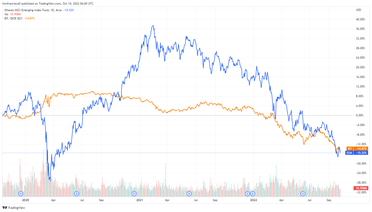
Some might wonder why DAA canaria cried from 2021. Answer to this question can be found at last image. Blue line represents emerging market index and orange line represents US long treasury index. As you can see, treasury makes negative signal from late 2020. And emerging market makes consistent bear signal from 2021. So the strategy kept portfolio to risk free asset classes.